Fitting and inference

This guide explains estimation and interpretation after the Get started workflow. See Extended examples for model specifications and Computation for engines, gradients and Jacobians.

Working example

The following bivariate model supplies the data used below.

library(emhawkes)

h <- new("hspec",
  mu = c(0.2, 0.2),
  alpha = matrix(c(0.5, 0.9, 0.9, 0.5), 2, byrow = TRUE),
  beta = matrix(2.25, 2, 2)
)
set.seed(1107)
path <- hsim(h, size = 1000)
#> Initial intensity components: auto -> mean (unconditional component means).
fit <- hfit(h, path$inter_arrival, path$type)
#> Initial intensity components: auto -> mean (unconditional component means).
#> hfit: equal starting values within each matrix share a parameter (reduced = TRUE; mu, alpha, beta).
#> Use reduced = FALSE to estimate matrix entries separately.
summary(fit)
#> --------------------------------------------
#> Maximum Likelihood estimation
#> BFGS maximization, 33 iterations
#> Return code 0: successful convergence 
#> Log-Likelihood: -970.1408 
#> 4  free parameters
#> Estimates:
#>          Estimate Std. error t value  Pr(> t)    
#> mu1       0.19095    0.01638  11.656  < 2e-16 ***
#> alpha1.1  0.48217    0.07430   6.489 8.64e-11 ***
#> alpha1.2  0.98625    0.09576  10.300  < 2e-16 ***
#> beta1.1   2.07987    0.17203  12.091  < 2e-16 ***
#> ---
#> Signif. codes:  0 '***' 0.001 '**' 0.01 '*' 0.05 '.' 0.1 ' ' 1
#> --------------------------------------------

Parameter sharing and fixed entries

By default, reduced = TRUE treats equal starting values within each parameter matrix as one parameter. This example estimates four parameters: one for mu, two for alpha, and one for beta. hfit() explains this rule once before optimization.

Use reduced = FALSE to estimate the ten matrix entries separately, even when their starting values are equal. Function components share parameters by name under either setting. A zero in a numeric matrix is also a starting value; use a component function to fix selected entries at zero.

The following examples show how starting values change the parameter map.

hspec2 <- h
res2 <- path

The sharing rule is applied separately to each matrix; equal values in mu and alpha do not link those components. The startup message lists matrices with shared entries. Use suppressMessages(hfit(...)) to hide it.

For example, if alpha[1,1] and alpha[1,2] have different initial values, hfit estimates them separately. If they have the same initial value, hfit treats them as a single parameter.

The previous example uses a symmetric Hawkes model: alpha is symmetric, and all entries of beta are equal.

print(hspec2)
#> An object of class "hspec" of 2-dimensional Hawkes process
#> 
#> Slot mu: 
#>      [,1]
#> [1,]  0.2
#> [2,]  0.2
#> 
#> Slot alpha: 
#>      [,1] [,2]
#> [1,]  0.5  0.9
#> [2,]  0.9  0.5
#> 
#> Slot beta: 
#>      [,1] [,2]
#> [1,] 2.25 2.25
#> [2,] 2.25 2.25

set.seed(1107)
res2 <- hsim(hspec2, size = 1000)
#> Initial intensity components: auto -> mean (unconditional component means).

In the first example, all entries of alpha0 are set to 0.75. This constrains alpha11, alpha12, alpha21, and alpha22 to share one estimated value, even though their simulation values differ. The same rule applies within mu0 and beta0.

mu0 <- matrix(c(0.15, 0.15), nrow = 2)
alpha0 <- matrix(c(0.75, 0.75, 0.75, 0.75), nrow = 2, byrow=TRUE)
beta0 <- matrix(c(2.6, 2.6, 2.6, 2.6), nrow = 2, byrow=TRUE)

hspec0 <- new("hspec", mu=mu0, alpha=alpha0, beta=beta0)
summary(hfit(hspec0, inter_arrival = res2$inter_arrival, type = res2$type))
#> Initial intensity components: auto -> mean (unconditional component means).
#> hfit: equal starting values within each matrix share a parameter (reduced = TRUE; mu, alpha, beta).
#> Use reduced = FALSE to estimate matrix entries separately.
#> --------------------------------------------
#> Maximum Likelihood estimation
#> BFGS maximization, 46 iterations
#> Return code 0: successful convergence 
#> Log-Likelihood: -979.5687 
#> 3  free parameters
#> Estimates:
#>          Estimate Std. error t value Pr(> t)    
#> mu1       0.19125    0.01633   11.71  <2e-16 ***
#> alpha1.1  0.73981    0.05783   12.79  <2e-16 ***
#> beta1.1   2.09707    0.15936   13.16  <2e-16 ***
#> ---
#> Signif. codes:  0 '***' 0.001 '**' 0.01 '*' 0.05 '.' 0.1 ' ' 1
#> --------------------------------------------

This fit estimates one excitation parameter for both self-excitation and mutual excitation, whose simulation values are 0.5 and 0.9, respectively.

In the second example, alpha0 has the same symmetry as the simulation model. Its diagonal entries are equal, and its off-diagonal entries share a different value. The model therefore has two excitation parameters to estimate.

mu0 <- matrix(c(0.15, 0.15), nrow = 2)
alpha0 <- matrix(c(0.75, 0.751, 0.751, 0.75), nrow = 2, byrow=TRUE)
beta0 <- matrix(c(2.6, 2.6, 2.6, 2.6), nrow = 2, byrow=TRUE)

hspec0 <- new("hspec", mu=mu0, alpha=alpha0, beta=beta0)
summary(hfit(hspec0, inter_arrival = res2$inter_arrival, type = res2$type))
#> Initial intensity components: auto -> mean (unconditional component means).
#> hfit: equal starting values within each matrix share a parameter (reduced = TRUE; mu, alpha, beta).
#> Use reduced = FALSE to estimate matrix entries separately.
#> --------------------------------------------
#> Maximum Likelihood estimation
#> BFGS maximization, 30 iterations
#> Return code 0: successful convergence 
#> Log-Likelihood: -970.1408 
#> 4  free parameters
#> Estimates:
#>          Estimate Std. error t value  Pr(> t)    
#> mu1       0.19095    0.01639  11.647  < 2e-16 ***
#> alpha1.1  0.48226    0.07292   6.614 3.74e-11 ***
#> alpha1.2  0.98626    0.09287  10.620  < 2e-16 ***
#> beta1.1   2.08008    0.16593  12.536  < 2e-16 ***
#> ---
#> Signif. codes:  0 '***' 0.001 '**' 0.01 '*' 0.05 '.' 0.1 ' ' 1
#> --------------------------------------------

The third example allows mu1 and mu2 to differ, even though they are equal in the simulation model.

mu0 <- matrix(c(0.15, 0.14), nrow = 2)
alpha0 <- matrix(c(0.75, 0.751, 0.751, 0.75), nrow = 2, byrow=TRUE)
beta0 <- matrix(c(2.6, 2.6, 2.6, 2.6), nrow = 2, byrow=TRUE)

hspec0 <- new("hspec", mu=mu0, alpha=alpha0, beta=beta0)
summary(hfit(hspec0, inter_arrival = res2$inter_arrival, type = res2$type))
#> Initial intensity components: auto -> mean (unconditional component means).
#> hfit: equal starting values within each matrix share a parameter (reduced = TRUE; alpha, beta).
#> Use reduced = FALSE to estimate matrix entries separately.
#> --------------------------------------------
#> Maximum Likelihood estimation
#> BFGS maximization, 42 iterations
#> Return code 0: successful convergence 
#> Log-Likelihood: -969.9914 
#> 5  free parameters
#> Estimates:
#>          Estimate Std. error t value Pr(> t)    
#> mu1       0.18300    0.02157   8.484  <2e-16 ***
#> mu2       0.19872    0.02206   9.006  <2e-16 ***
#> alpha1.1  0.48149    0.07569   6.361   2e-10 ***
#> alpha1.2  0.98720    0.09852  10.020  <2e-16 ***
#> beta1.1   2.07973    0.17931  11.598  <2e-16 ***
#> ---
#> Signif. codes:  0 '***' 0.001 '**' 0.01 '*' 0.05 '.' 0.1 ' ' 1
#> --------------------------------------------

Set reduced = FALSE to estimate each matrix entry separately, including entries with equal initial values.

summary(hfit(hspec2, inter_arrival = res2$inter_arrival, type = res2$type, reduced=FALSE))
#> Initial intensity components: auto -> mean (unconditional component means).
#> hfit: some standard errors are NaN. Try final_hessian = "stable" for Hawkes Hessian diagnostics, then inspect fit_diagnostics().
#> --------------------------------------------
#> Maximum Likelihood estimation
#> BFGS maximization, 51 iterations
#> Return code 0: successful convergence 
#> Log-Likelihood: -966.5055 
#> 10  free parameters
#> Estimates:
#>          Estimate Std. error t value  Pr(> t)    
#> mu1       0.17997    0.02231   8.066 7.24e-16 ***
#> mu2       0.20060    0.02335   8.590  < 2e-16 ***
#> alpha1.1  0.44726    0.10661   4.195 2.73e-05 ***
#> alpha2.1  1.17743        NaN     NaN      NaN    
#> alpha1.2  0.97048    0.10742   9.035  < 2e-16 ***
#> alpha2.2  0.48979        NaN     NaN      NaN    
#> beta1.1   2.52210        NaN     NaN      NaN    
#> beta2.1   3.15498        NaN     NaN      NaN    
#> beta1.2   1.80167    0.07600  23.705  < 2e-16 ***
#> beta2.2   1.51338        NaN     NaN      NaN    
#> ---
#> Signif. codes:  0 '***' 0.001 '**' 0.01 '*' 0.05 '.' 0.1 ' ' 1
#> --------------------------------------------

The same rules apply to higher-dimensional models. For function components, the named entries in param define the estimated parameters. Matching parameter names are shared across functions, even with reduced = FALSE. Use different names for independent parameters with equal starting values. Conflicting starting values for a shared name produce a warning, and the first value is used. A zero in a numeric matrix is an estimated starting value; constants inside a component function remain fixed.

Observed data and initial state

The first data row is the initial state. inter_arrival, type, and mark start with zero, followed by the observed events. hsim(size) includes this initial row. N0 and Nc0 specify initial counts and mark totals; Nc0 must be named in hfit().

The likelihood ends at the last supplied event. N0 and Nc0 accept a scalar or one value per event type. Supplied N and Nc matrices must agree with the event data and initial counts. Explicit type_col_map requires initial kernel components for simulation and the built-in likelihood.

Event order is preserved when times coincide. Use the same initial counts and lambda_component0 for simulation and likelihood evaluation when comparing paths. A scalar lambda_component0 is expanded to all kernel components; a matrix must match the kernel dimensions. For multi-kernel models, supply it explicitly.

Counting-process matrices supplied as N or Nc must agree with the event data and initial counts. Each row contains the values after that event. A baseline function called with index n uses row n - 1 for the preceding state; an impact function uses row n for the current event. Component functions can declare only the arguments they need, and use ... to receive the remaining context.

Prepare observed event times measured from the observation start as follows:

inter_arrival <- c(0, diff(c(0, event_times)))
type <- c(0, event_types)
mark <- c(0, event_marks)

Omit type for a univariate model and mark for unit marks. The vectors must have the same length; event types range from 1 to the model dimension.

Restoring and saving a fitted model

Use fitted_hspec(fit) to restore the estimated model and fit_initial_state(fit) to retrieve the initial-state arguments:

estimated <- fitted_hspec(fit)
initial <- fit_initial_state(fit)
inferred <- do.call(logLik, c(list(object = estimated,
  inter_arrival = path$inter_arrival, type = path$type, mark = path$mark,
  infer = TRUE), initial))
#> Initial intensity components: mean (unconditional component means).

The result remains a maxLik object, so coef(), summary(), and vcov() keep their existing behavior. The saved parameter map preserves shared parameters and fixed constants in component functions. Simulation generators are retained, and their named parameters are updated when they match estimated coefficient names. Automatic initial intensity remains NULL and is recalculated for the restored model. Initial counts are retained. A custom objective is not incorporated into the restored model.

Save the fit with saveRDS() to retain this information between sessions. Keep the observed data separately and supply them again for inference. The stored optimization objective can retain data in its function environment. The saved initial state describes the start of the observation window. Pass it to hsim() to start a new path from the estimated model. Continuing after the last observed event requires that event’s state. Fits created without the new metadata need to be refitted before using the reconstruction helpers.

Pass the restored specification and the saved initial-state arguments to hsim() to generate a new path after checking convergence and model suitability.

set.seed(1108)
simulated <- do.call(hsim, c(list(object = estimated, size = 100), initial))
head(simulated$arrival)
#> [1] 0.000000 2.526746 2.946904 3.216280 3.253234 4.359288

saveRDS(fit, "hawkes-fit.rds")
saved_fit <- readRDS("hawkes-fit.rds")
estimated <- fitted_hspec(saved_fit)
initial <- fit_initial_state(saved_fit)

Curvature and standard errors

By default, hfit() uses the final Hessian and standard errors from maxLik. It does not run the additional stabilization checks. If numerical Hawkes standard errors contain NaN, a short message suggests trying final_hessian = "stable". Request this option to check numerical Hawkes curvature with scaled central differences and Richardson extrapolation. With auto or cpp, stable curvature differentiates the built-in analytic score when the model is supported and any required component Jacobians are supplied. This also works with the default numerical optimizer gradient. Unsupported score models, missing Jacobians, or failed score evaluations use likelihood differences; r always uses likelihood differences. Inspect curvature_source and score_fallback_reason in fit_diagnostics(fit) for the selected path. This preserves the optimizer’s coefficients and log-likelihood. summary() and vcov() then use the checked covariance; free-parameter standard errors are NA when stable inversion is unavailable. Inspect fit_diagnostics(fit) for the requested checks. Supplied Hessians, disabled final curvature, BHHH, custom objectives, and residual models retain their calculation choices.

For unconstrained BFGS, CG, Nelder-Mead, and SANN fits without supplied hess or finalHessian, stable curvature omits maxLik’s separate final Hessian. Inspect fit_diagnostics(fit)$computation$hessian$maxLik_skipped; the omitted matrix is not stored in original_hessian. Use finalHessian = TRUE to retain that extra calculation. The default final_hessian = "maxLik" is unchanged.

A stable Hessian does not guarantee reliable Wald intervals. Nearby kernel decay rates, weak excitation, boundaries, short samples, and nonsmooth callbacks can still make inference unreliable. The Hawkes standard-error report compares unchanged estimates and corrected standard errors, and discusses profile likelihood and bootstrap. The earlier diagnostic report records the original Hawkes and FRPP issues.

Check convergence, score, and multiple starting values before interpreting intervals.

For otherwise identical kernels driven by the same events, equal decay rates can leave only the combined amplitude identifiable. Small excitation alone does not require missing standard errors: known initial excitation can still carry decay information. See the Hawkes curvature stress checks.

For checked fits, an unsuccessful optimizer triggers a warning even when stable curvature is unavailable. Inspect optimizer_success, optimizer_code and warnings in fit_diagnostics(fit) alongside its curvature status and reason.

fit_checked <- hfit(h, path$inter_arrival, path$type, final_hessian = "stable")
#> Initial intensity components: auto -> mean (unconditional component means).
#> hfit: equal starting values within each matrix share a parameter (reduced = TRUE; mu, alpha, beta).
#> Use reduced = FALSE to estimate matrix entries separately.
fit_diagnostics(fit_checked)[c("status", "scaled_condition", "newton_decrement")]
#> $status
#> [1] "ok"
#> 
#> $scaled_condition
#> [1] 25.35156
#> 
#> $newton_decrement
#> [1] 8.296909e-06

The calculation record is explained in Computation.

Residual diagnostics

logLik(h, ..., infer = TRUE) returns a list with the likelihood, intensity paths, and residual vectors. Use it in place of the deprecated infer_lambda() and residual_process() helpers. Simulation returns an hreal object.

Set infer = TRUE in logLik to obtain the log-likelihood, intensity paths, and residual processes. These are computed using the parameters in the supplied hspec object. For a univariate model, res_process1 contains the residual inter-arrival times.

hrp <- new("hspec", mu = 0.3, alpha = 1.2, beta = 1.5)
res_rp <- hsim(hrp, size = 1000)

# inferred result
infered_res <- logLik(hrp, res_rp$inter_arrival, infer = TRUE)

## QQ-plot
p <- ppoints(100)
q <- quantile(infered_res$res_process1, p = p)
plot(qexp(p), q, xlab="Theoretical Quantiles",ylab="Sample Quantiles")
qqline(q, distribution=qexp,col="blue", lty=2)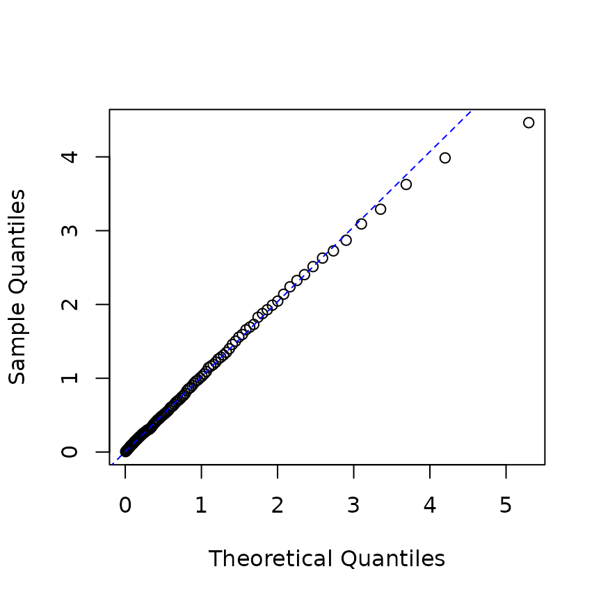

For observed data, estimate the parameters before computing the residual processes.


# estimation
mle_rp <- hfit(new("hspec", mu = 0.2, alpha = 1, beta = 2),
               res_rp$inter_arrival)

# Restore the estimated model and the initial-state arguments.
he <- fitted_hspec(mle_rp)
initial_rp <- fit_initial_state(mle_rp)

# infer intensity
infered_res <- do.call(logLik, c(list(object = he,
  inter_arrival = res_rp$inter_arrival, type = res_rp$type, infer = TRUE), initial_rp))

rpe <- infered_res$res_process1

p <- ppoints(100)
q <- quantile(rpe, p=p)
plot(qexp(p), q, xlab="Theoretical Quantiles",ylab="Sample Quantiles")
qqline(q, distribution=qexp,col="blue", lty=2)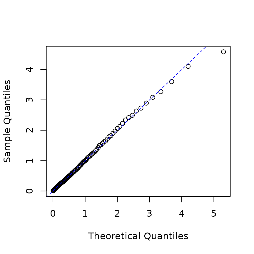

For an $n$ -dimensional model, logLik returns one residual process for each event type. In the following bivariate example, these are infer_res2$res_process1 and infer_res2$res_process2.

hrp2 <- new("hspec", mu = rep(0.3, 2),
           alpha = matrix(c(1.2, 1.5, 1.5, 1.2), nrow=2),
           beta = matrix(rep(3, 4), nrow=2))
res_hrp2 <- hsim(hrp2, size = 2000)

infer_res2 <- logLik(hrp2, res_hrp2$inter_arrival, res_hrp2$type, infer = TRUE)

p <- ppoints(100)
q <- quantile(c(infer_res2$res_process1, infer_res2$res_process2), p=p)
plot(qexp(p), q, xlab="Theoretical Quantiles",ylab="Sample Quantiles")
qqline(q, distribution=qexp,col="blue", lty=2)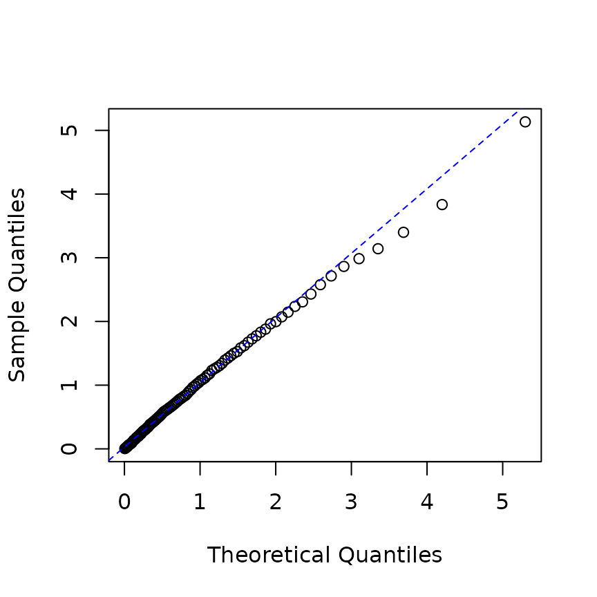

# Plot the pooled residuals for both event types.

hist(
  c(infer_res2$res_process1, infer_res2$res_process2),
  breaks = 50,
  probability = TRUE,
  main = "Histogram of Inferred Residual Process",
  xlab = "Residual Value",
  ylab = "Density"
)

x <- seq(0, 8, 0.1)

lines(
  x,
  dexp(x),
  col = 'red',
  lwd = 2
)

legend("topright", legend = "Theoretical PDF", col = "red", lwd = 2)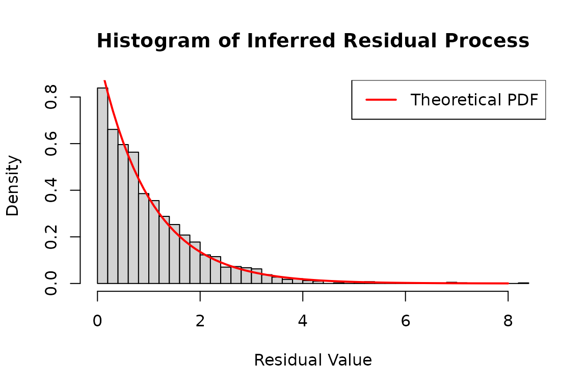

Residual checks assess model adequacy; they do not replace convergence or curvature checks. See the flexible residual examples for models with a non-exponential residual law.