Extended example : emhawkes package

Kyungsub Lee

2025-08-26

Basic Hawkes model

Univariate Hawkes process

library(emhawkes)

This subsection outlines the steps for constructing, running simulations, and estimating a univariate Hawkes model. To begin, create an hspec object, which defines the Hawkes model. The S4 class hspec contains slots for the model parameters: mu, alpha, beta, dimens, rmark, and impact.

In a univariate model, the basic parameters of the model—mu, alpha, and beta—can be given as numeric values. If numeric values are provided, they will be converted to matrices. Below is an example of a univariate Hawkes model without a mark.

mu1 <- 0.3; alpha1 <- 1.2; beta1 <- 1.5
hspec1 <- new("hspec", mu = mu1, alpha = alpha1, beta = beta1)
show(hspec1)
#> An object of class "hspec" of 1-dimensional Hawkes process
#> 
#> Slot mu: 
#>      [,1]
#> [1,]  0.3
#> 
#> Slot alpha: 
#>      [,1]
#> [1,]  1.2
#> 
#> Slot beta: 
#>      [,1]
#> [1,]  1.5

The function hsim implements simulation where the input arguments are hspec, size, and the initial values of the intensity component process, lambda_component0, and the initial values of the Hawkes processes, N0. More precisely, the intensity process of the basic univariate Hawkes model is represented by

$$\lambda(t) = \mu + \int_{-\infty}^t \alpha e^{-\beta (t-s)} d N(s) = \mu + \lambda_c(0) e^{-\beta t} + \int_0^t \alpha e^{-\beta (t-s)} d N(s)$$

where the lambda_component0 denotes

$$\lambda_c(0) = \int_{-\infty}^0 \alpha e^{\beta s} d N(s).$$

If lambda_component0 is not provided, the internally determined initial values for the intensity process are used. If size is sufficiently large, the exact value of lambda_component0 may not be important. The default initial value of the counting process, N0, is zero.

set.seed(1107)
res1 <- hsim(hspec1, size = 1000)
summary(res1)
#> -------------------------------------------------------
#> Simulation result of exponential (marked) Hawkes model.
#> Realized path :
#>        arrival N1 mark lambda1
#>  [1,]  0.00000  0    0 0.90000
#>  [2,]  0.97794  1    1 0.43838
#>  [3,]  1.09001  2    1 1.43128
#>  [4,]  1.28999  3    1 2.02711
#>  [5,]  1.53225  4    1 2.33527
#>  [6,]  1.65001  5    1 3.01139
#>  [7,]  2.51807  6    1 1.36377
#>  [8,]  2.81710  7    1 1.74553
#>  [9,]  2.87547  8    1 2.72378
#> [10,]  3.16415  9    1 2.65016
#> [11,]  3.51378 10    1 2.40131
#> [12,]  4.22355 11    1 1.43843
#> [13,] 16.96752 12    1 0.30000
#> [14,] 17.71654 13    1 0.69015
#> [15,] 19.10293 14    1 0.49874
#> [16,] 24.06354 15    1 0.30082
#> [17,] 24.09256 16    1 1.44967
#> [18,] 28.40173 17    1 0.30366
#> [19,] 28.53743 18    1 1.28198
#> [20,] 28.56702 19    1 2.38725
#> ... with 980 more rows 
#> -------------------------------------------------------

The results of hsim is an S3 class hreal, which consists of hspec, inter_arrival, arrival, type, mark, N, Nc, lambda, lambda_component, rambda, rambda_component.

• hspec is the model specification.

• inter_arrival is the inter-arrival time of every event.

• arrival is the cumulative sum of inter_arrival.

• type is the type of events, i.e., $i$ for $N_i$, and is used for a multivariate model.

• mark is a numeric vector that represents additional information for the event.

• lambda represents $\lambda$, which is the left continuous and right limit version.

• The right continuous version of intensity is rambda.

• lambda_component represents $\lambda_{ij}$, and rambda_component is the right continuous version.

inter_arrival, type, mark, N, and Nc start at zero. Using the summary() function, one can print the first 20 elements of arrival, N, and lambda. The print() function can also be used.

By definition, we have lambda == mu + lambda_component.

# first and third columns are the same
cbind(res1$lambda[1:5], res1$lambda_component[1:5], mu1 + res1$lambda_component[1:5])
#>          [,1]     [,2]     [,3]
#> [1,] 0.900000 0.600000 0.900000
#> [2,] 0.438383 0.138383 0.438383
#> [3,] 1.431282 1.131282 1.431282
#> [4,] 2.027111 1.727111 2.027111
#> [5,] 2.335269 2.035269 2.335269

For all rows except the first, rambda equals lambda + alpha in this model.

# second and third columns are the same
cbind(res1$lambda[1:5], res1$rambda[1:5], res1$lambda[1:5] + alpha1)
#>          [,1]     [,2]     [,3]
#> [1,] 0.900000 0.900000 2.100000
#> [2,] 0.438383 1.638383 1.638383
#> [3,] 1.431282 2.631282 2.631282
#> [4,] 2.027111 3.227111 3.227111
#> [5,] 2.335269 3.535269 3.535269

Additionally, verify that the exponential decay is accurately represented in the model.

# By definition, the following two are equal:
res1$lambda[2:6]
#> [1] 0.438383 1.431282 2.027111 2.335269 3.011391
mu1 + (res1$rambda[1:5] - mu1) * exp(-beta1 * res1$inter_arrival[2:6])
#> [1] 0.438383 1.431282 2.027111 2.335269 3.011391

The log-likelihood function is calculated using the logLik method. In this context, the inter-arrival times and hspec are provided as inputs to the function.

logLik(hspec1, inter_arrival = res1$inter_arrival)
#> The initial values for intensity processes are not provided. Internally determined initial values are used.
#> loglikelihood 
#>     -214.2385

The likelihood estimation is performed using the hfit function. The specification of the initial parameter values, hspec0, is required. Note that only inter_arrival is needed for this univariate model. For more accurate simulation, it is recommended to specify lambda0, the initial value of the lambda component. If lambda0 is not provided, the function uses internally determined initial values. By default, the BFGS method is employed for numerical optimization.

# initial value for numerical optimization
mu0 <- 0.5; alpha0 <- 1.0; beta0 <- 1.8
hspec0 <- new("hspec", mu = mu0, alpha = alpha0, beta = beta0)
# the intial values are provided through hspec
mle <- hfit(hspec0, inter_arrival = res1$inter_arrival)
summary(mle)
#> --------------------------------------------
#> Maximum Likelihood estimation
#> BFGS maximization, 24 iterations
#> Return code 0: successful convergence 
#> Log-Likelihood: -213.4658 
#> 3  free parameters
#> Estimates:
#>        Estimate Std. error t value Pr(> t)    
#> mu1     0.33641    0.03475   9.682  <2e-16 ***
#> alpha1  1.16654    0.09608  12.141  <2e-16 ***
#> beta1   1.52270    0.12468  12.213  <2e-16 ***
#> ---
#> Signif. codes:  0 '***' 0.001 '**' 0.01 '*' 0.05 '.' 0.1 ' ' 1
#> --------------------------------------------

Bivariate Hawkes model

The intensity process of a basic bivariate Hawkes model is defined by

$$\lambda_1(t) = \mu_1 + \int_{-\infty}^t \alpha_{11} e^{-\beta_{11}(t-s)} d N_1(s) + \int_{-\infty}^t \alpha_{12} e^{-\beta_{12}(t-s)} d N_2(s),$$

$$\lambda_2(t) = \mu_2 + \int_{-\infty}^t \alpha_{21} e^{-\beta_{21}(t-s)} d N_1(s) + \int_{-\infty}^t \alpha_{22} e^{-\beta_{22}(t-s)} d N_2(s).$$

In a bivariate model, the parameters within the slots of hspec are matrices. Specifically, mu is a 2-by-1 matrix, while alpha and beta are 2-by-2 matrices.

$$\mu = \begin{bmatrix} \mu_1 \\ \mu_2 \end{bmatrix}, \quad \alpha = \begin{bmatrix} \alpha_{11} & \alpha_{12} \\ \alpha_{21} & \alpha_{22} \end{bmatrix}, \quad \beta = \begin{bmatrix} \beta_{11} & \beta_{12} \\ \beta_{21} & \beta_{22} \end{bmatrix}$$

rmark is a random number generating function for marks and is not used in non-mark models. lambda_component0 is a 2-by-2 matrix that represents the initial values of lambda_component, which includes the set of values lambda11, lambda12, lambda21, and lambda22. The intensity processes are represented by

$$\lambda_1(t) = \mu_1 + \lambda_{11}(t) + \lambda_{12}(t),$$

$$\lambda_2(t) = \mu_2 + \lambda_{21}(t) + \lambda_{22}(t).$$

The terms $\lambda_{ij}$ are referred to as lambda components, and lambda0 represents $_{ij}(0). The parameterlambda_component0` can be omitted in this model, in which case internally determined initial values will be used.

mu2 <- matrix(c(0.2), nrow = 2)
alpha2 <- matrix(c(0.5, 0.9, 0.9, 0.5), nrow = 2, byrow = TRUE)
beta2 <- matrix(c(2.25, 2.25, 2.25, 2.25), nrow = 2, byrow = TRUE)
hspec2 <- new("hspec", mu=mu2, alpha=alpha2, beta=beta2)
print(hspec2)
#> An object of class "hspec" of 2-dimensional Hawkes process
#> 
#> Slot mu: 
#>      [,1]
#> [1,]  0.2
#> [2,]  0.2
#> 
#> Slot alpha: 
#>      [,1] [,2]
#> [1,]  0.5  0.9
#> [2,]  0.9  0.5
#> 
#> Slot beta: 
#>      [,1] [,2]
#> [1,] 2.25 2.25
#> [2,] 2.25 2.25

To perform a simulation, use the hsim function.

set.seed(1107)
res2 <- hsim(hspec2,  size=1000)
summary(res2)
#> -------------------------------------------------------
#> Simulation result of exponential (marked) Hawkes model.
#> Realized path :
#>       arrival N1 N2 mark lambda1 lambda2
#>  [1,] 0.00000  0  0    0 0.52941 0.52941
#>  [2,] 0.57028  1  0    1 0.29130 0.29130
#>  [3,] 1.66175  1  1    1 0.25073 0.28505
#>  [4,] 2.17979  1  2    1 0.49638 0.38238
#>  [5,] 2.47685  1  3    1 0.81319 0.54975
#>  [6,] 2.64001  2  3    1 1.24825 0.78866
#>  [7,] 2.70249  3  3    1 1.54519 1.49341
#>  [8,] 2.94547  4  3    1 1.26810 1.46968
#>  [9,] 3.39313  4  4    1 0.77271 0.99242
#> [10,] 3.52533  4  5    1 1.29379 1.15989
#> [11,] 3.56971  5  5    1 2.00432 1.52115
#> [12,] 3.70761  5  6    1 1.88965 1.82866
#> [13,] 4.30122  5  7    1 0.88106 0.75983
#> [14,] 4.34337  6  7    1 1.63800 1.16393
#> [15,] 4.40222  7  7    1 1.89764 1.83275
#> [16,] 4.58943  8  7    1 1.64219 1.86211
#> [17,] 5.14665  9  7    1 0.75437 0.93131
#> [18,] 5.18186  9  8    1 1.17407 1.70707
#> [19,] 5.36167  9  9    1 1.45050 1.53925
#> [20,] 5.89118 10  9    1 0.85331 0.75875
#> ... with 980 more rows 
#> -------------------------------------------------------

In multivariate models, type is crucial as it represents the type of event.

# Under bi-variate model, there are two types, 1 or 2.
res2$type[1:10]
#>  [1] 0 1 2 2 2 1 1 1 2 2

In multivariate models, the column names of N are N1, N2, N3, and so on.

res2$N[1:3, ]
#>      N1 N2
#> [1,]  0  0
#> [2,]  1  0
#> [3,]  1  1

Similarly, the column names of lambda are lambda1, lambda2, lambda3, and so on.

res2$lambda[1:3, ]
#>        lambda1   lambda2
#> [1,] 0.5294118 0.5294118
#> [2,] 0.2913028 0.2913028
#> [3,] 0.2507301 0.2850475

The column names of lambda_component are lambda_component11, lambda_component12, lambda_component13, and so on.

res2$lambda_component[1:3, ]
#>        lambda11    lambda12   lambda21    lambda22
#> [1,] 0.11764706 0.211764706 0.21176471 0.117647059
#> [2,] 0.03260813 0.058694641 0.05869464 0.032608134
#> [3,] 0.04569443 0.005035631 0.08224997 0.002797573

By definition, the following two expressions are equivalent:

mu2[1] + rowSums(res2$lambda_component[1:5, c("lambda11", "lambda12")])
#> [1] 0.5294118 0.2913028 0.2507301 0.4963769 0.8131889
res2$lambda[1:5, "lambda1"]
#> [1] 0.5294118 0.2913028 0.2507301 0.4963769 0.8131889

From the results, we obtain vectors of realized inter_arrival and type. A bivariate model requires both inter_arrival and type for estimation.

inter_arrival2 <- res2$inter_arrival
type2 <- res2$type

The log-likelihood is computed using the logLik function.

logLik(hspec2, inter_arrival = inter_arrival2, type = type2)
#> The initial values for intensity processes are not provided. Internally determined initial values are used.
#> loglikelihood 
#>     -974.2809

Maximum log-likelihood estimation is performed using the hfit function. In this process, the parameter values in hspec0, such as mu, alpha, and beta, serve as starting points for the numerical optimization. For illustration purposes, we set hspec0 <- hspec2. Since the true parameter values are unknown in practical applications, these initial guesses are used. The realized inter_arrival and type data are utilized for estimation.

hspec0 <- hspec2
mle <- hfit(hspec0, inter_arrival = inter_arrival2, type = type2)
summary(mle)
#> --------------------------------------------
#> Maximum Likelihood estimation
#> BFGS maximization, 36 iterations
#> Return code 0: successful convergence 
#> Log-Likelihood: -970.1408 
#> 4  free parameters
#> Estimates:
#>          Estimate Std. error t value  Pr(> t)    
#> mu1       0.19095    0.01636  11.671  < 2e-16 ***
#> alpha1.1  0.48217    0.07405   6.511 7.45e-11 ***
#> alpha1.2  0.98625    0.09495  10.387  < 2e-16 ***
#> beta1.1   2.07987    0.16952  12.269  < 2e-16 ***
#> ---
#> Signif. codes:  0 '***' 0.001 '**' 0.01 '*' 0.05 '.' 0.1 ' ' 1
#> --------------------------------------------

coef(mle)
#>       mu1  alpha1.1  alpha1.2   beta1.1 
#> 0.1909541 0.4821725 0.9862542 2.0798691

miscTools::stdEr(mle)
#>        mu1   alpha1.1   alpha1.2    beta1.1 
#> 0.01636127 0.07405118 0.09495461 0.16952428

Parameter setting

This subsection explores the relationship between parameter settings and the estimation procedure in a multivariate Hawkes model. The number of parameters to be estimated in the model is influenced by how we configure parameter slots such as mu, alpha, and beta in hspec0, which specifies the initial values.

Since the parameter slot alpha is a matrix, its elements can either be the same or different. Consequently, the number of parameters estimated varies depending on whether the initial settings have identical or distinct elements.

For example, if alpha[1,1] and alpha[1,2] in hspec0 are initially set to different values, the numerical procedure will estimate alpha[1,1] and alpha[1,2] separately. Conversely, if alpha[1,1] and alpha[1,2] are the same in the initial setting, the estimation procedure treats these parameters as identical in the model, thus estimating only one value.

Recall that the example in the previous section features a symmetric Hawkes model, where the matrix alpha is symmetric and all elements of beta are identical.

print(hspec2)
#> An object of class "hspec" of 2-dimensional Hawkes process
#> 
#> Slot mu: 
#>      [,1]
#> [1,]  0.2
#> [2,]  0.2
#> 
#> Slot alpha: 
#>      [,1] [,2]
#> [1,]  0.5  0.9
#> [2,]  0.9  0.5
#> 
#> Slot beta: 
#>      [,1] [,2]
#> [1,] 2.25 2.25
#> [2,] 2.25 2.25

set.seed(1107)
res2 <- hsim(hspec2, size = 1000)

In the first estimation example, the initial value of alpha0 is a matrix where all elements are set to the same value of 0.75. In this configuration, hfit assumes that alpha11, alpha12, alpha21, and alpha22 are identical in the model, even if the actual parameters have different values. Similarly, the parameter matrices mu0 and beta0 are treated in the same manner.

mu0 <- matrix(c(0.15, 0.15), nrow = 2)
alpha0 <- matrix(c(0.75, 0.75, 0.75, 0.75), nrow = 2, byrow=TRUE)
beta0 <- matrix(c(2.6, 2.6, 2.6, 2.6), nrow = 2, byrow=TRUE)

hspec0 <- new("hspec", mu=mu0, alpha=alpha0, beta=beta0)
summary(hfit(hspec0, inter_arrival = res2$inter_arrival, type = res2$type))
#> --------------------------------------------
#> Maximum Likelihood estimation
#> BFGS maximization, 44 iterations
#> Return code 0: successful convergence 
#> Log-Likelihood: -979.5687 
#> 3  free parameters
#> Estimates:
#>          Estimate Std. error t value Pr(> t)    
#> mu1       0.19125    0.01636   11.69  <2e-16 ***
#> alpha1.1  0.73981    0.05951   12.43  <2e-16 ***
#> beta1.1   2.09707    0.16524   12.69  <2e-16 ***
#> ---
#> Signif. codes:  0 '***' 0.001 '**' 0.01 '*' 0.05 '.' 0.1 ' ' 1
#> --------------------------------------------

Note that in the above result, alpha1.1 falls somewhere between the original values of alpha1.1 = 0.5 and alpha1.2 = 0.9.

In the following second example, the elements of alpha0 are not identical but are symmetric, reflecting the original values used in the simulation. Specifically, we have alpha11 == alpha22 and alpha12 == alpha21 in alpha0, so alpha11 and alpha12 will be estimated differently.

mu0 <- matrix(c(0.15, 0.15), nrow = 2)
alpha0 <- matrix(c(0.75, 0.751, 0.751, 0.75), nrow = 2, byrow=TRUE)
beta0 <- matrix(c(2.6, 2.6, 2.6, 2.6), nrow = 2, byrow=TRUE)

hspec0 <- new("hspec", mu=mu0, alpha=alpha0, beta=beta0)
summary(hfit(hspec0, inter_arrival = res2$inter_arrival, type = res2$type))
#> --------------------------------------------
#> Maximum Likelihood estimation
#> BFGS maximization, 30 iterations
#> Return code 0: successful convergence 
#> Log-Likelihood: -970.1408 
#> 4  free parameters
#> Estimates:
#>          Estimate Std. error t value Pr(> t)    
#> mu1       0.19095    0.01643  11.619 < 2e-16 ***
#> alpha1.1  0.48226    0.07421   6.499 8.1e-11 ***
#> alpha1.2  0.98626    0.09538  10.341 < 2e-16 ***
#> beta1.1   2.08008    0.17303  12.021 < 2e-16 ***
#> ---
#> Signif. codes:  0 '***' 0.001 '**' 0.01 '*' 0.05 '.' 0.1 ' ' 1
#> --------------------------------------------

In the third example, the estimation is performed under the assumption that mu1 and mu2 may differ, even though they are the same in the original model.

mu0 <- matrix(c(0.15, 0.14), nrow = 2)
alpha0 <- matrix(c(0.75, 0.751, 0.751, 0.75), nrow = 2, byrow=TRUE)
beta0 <- matrix(c(2.6, 2.6, 2.6, 2.6), nrow = 2, byrow=TRUE)

hspec0 <- new("hspec", mu=mu0, alpha=alpha0, beta=beta0)
summary(hfit(hspec0, inter_arrival = res2$inter_arrival, type = res2$type))
#> --------------------------------------------
#> Maximum Likelihood estimation
#> BFGS maximization, 42 iterations
#> Return code 0: successful convergence 
#> Log-Likelihood: -969.9914 
#> 5  free parameters
#> Estimates:
#>          Estimate Std. error t value  Pr(> t)    
#> mu1       0.18300    0.02154   8.495  < 2e-16 ***
#> mu2       0.19872    0.02203   9.020  < 2e-16 ***
#> alpha1.1  0.48149    0.07425   6.484 8.91e-11 ***
#> alpha1.2  0.98720    0.09556  10.331  < 2e-16 ***
#> beta1.1   2.07973    0.17094  12.166  < 2e-16 ***
#> ---
#> Signif. codes:  0 '***' 0.001 '**' 0.01 '*' 0.05 '.' 0.1 ' ' 1
#> --------------------------------------------

By setting reduced = FALSE, all parameters are estimated.

summary(hfit(hspec2, inter_arrival = res2$inter_arrival, type = res2$type, reduced=FALSE))
#> --------------------------------------------
#> Maximum Likelihood estimation
#> BFGS maximization, 51 iterations
#> Return code 0: successful convergence 
#> Log-Likelihood: -966.5055 
#> 10  free parameters
#> Estimates:
#>          Estimate Std. error t value  Pr(> t)    
#> mu1       0.17997    0.02312   7.784 7.05e-15 ***
#> mu2       0.20060    0.02442   8.214  < 2e-16 ***
#> alpha1.1  0.44726    0.16627   2.690  0.00714 ** 
#> alpha2.1  1.17743    0.22909   5.140 2.75e-07 ***
#> alpha1.2  0.97048    0.14242   6.814 9.47e-12 ***
#> alpha2.2  0.48979    0.15398   3.181  0.00147 ** 
#> beta1.1   2.52210    1.16375   2.167  0.03022 *  
#> beta2.1   3.15498    0.67702   4.660 3.16e-06 ***
#> beta1.2   1.80167    0.25695   7.012 2.35e-12 ***
#> beta2.2   1.51338    0.54476   2.778  0.00547 ** 
#> ---
#> Signif. codes:  0 '***' 0.001 '**' 0.01 '*' 0.05 '.' 0.1 ' ' 1
#> --------------------------------------------

The same logic applies to all higher-dimensional models.

Residual process

The residual process can be extracted using the logLik() function by setting infer = TRUE. When this option is enabled, the logLik function returns a list that includes the log-likelihood, inferred intensities, and the residual process. Note that the inference is based on the object passed to the logLik function. In the returned object, res_process1 represents the residual process.

hrp <- new("hspec", mu = 0.3, alpha = 1.2, beta = 1.5)
res_rp <- hsim(hrp, size = 1000)

# inferred result
infered_res <- logLik(hrp, res_rp$inter_arrival, infer = TRUE)

## QQ-plot
p <- ppoints(100)
q <- quantile(infered_res$res_process1, p = p)
plot(qexp(p), q, xlab="Theoretical Quantiles",ylab="Sample Quantiles")
qqline(q, distribution=qexp,col="blue", lty=2)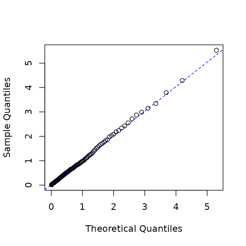

In practical scenarios, the parameter values are usually unknown, so the model may be estimated before computing the residual processes.

# estimation
mle_rp <- hfit(new("hspec", mu = 0.2, alpha = 1, beta = 2),
               res_rp$inter_arrival)

# construct hspec from estimation result
he <- new("hspec", mu = coef(mle_rp)["mu1"], 
          alpha = coef(mle_rp)["alpha1"], beta = coef(mle_rp)["beta1"])

# infer intensity
infered_res <- logLik(he, res_rp$inter_arrival, res_rp$type, infer = TRUE)

rpe <- infered_res$res_process1

p <- ppoints(100)
q <- quantile(rpe, p=p)
plot(qexp(p), q, xlab="Theoretical Quantiles",ylab="Sample Quantiles")
qqline(q, distribution=qexp,col="blue", lty=2)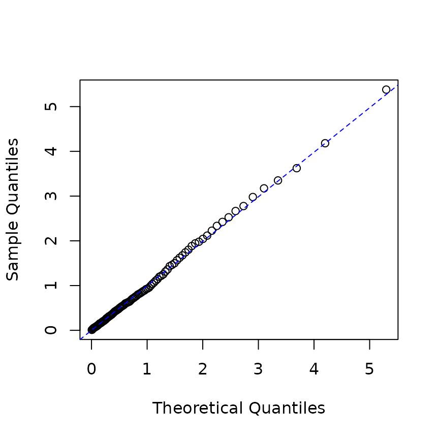

In an $n$-dimensional model, we can compute the residuals in a similar manner. In this case, the object returned by the logLik function contains $n$ residual processes. For example, in the following code, infer_res2$res_process1 and infer_res2$res_process2 represent the residual processes for each type.

hrp2 <- new("hspec", mu = rep(0.3, 2), 
           alpha = matrix(c(1.2, 1.5, 1.5, 1.2), nrow=2), 
           beta = matrix(rep(3, 4), nrow=2))
res_hrp2 <- hsim(hrp2, size = 2000)

infer_res2 <- logLik(hrp2, res_hrp2$inter_arrival, res_hrp2$type, infer = TRUE)

p <- ppoints(100)
q <- quantile(c(infer_res2$res_process1, infer_res2$res_process2), p=p)
plot(qexp(p), q, xlab="Theoretical Quantiles",ylab="Sample Quantiles")
qqline(q, distribution=qexp,col="blue", lty=2)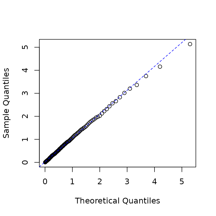

# Infer the residual process using the log-likelihood method
# 'infer_res_dh1' contains the inferred process data based on the inter-arrival times

hist(
  c(infer_res2$res_process1, infer_res2$res_process2),
  breaks = 50,
  probability = TRUE,
  main = "Histogram of Inferred Residual Process",
  xlab = "Residual Value",
  ylab = "Density"
)

x <- seq(0, 8, 0.1)

lines(
  x,
  dexp(x),
  col = 'red',
  lwd = 2
)

legend("topright", legend = "Theoretical PDF", col = "red", lwd = 2)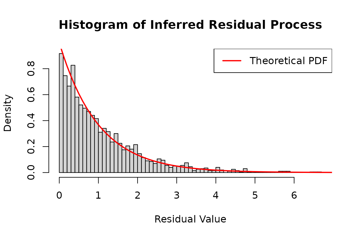

More complicated model

Multi-kernel model

In a multi-kernel Hawkes model, type_col_map is required for hspec. type_col_map is a list that represents the mapping between type and column number. For example, consider a bi-variate multi-kernel model: $$\lambda_t = \mu + \int_{-\infty}^{t} h(t-u) d N(u)$$ where $$h = \sum_{k=1}^{K} h_k, \quad h_k (t) = \alpha_k \circ \begin{bmatrix} e^{-\beta_{k11} t} & e^{-\beta_{k12} t} \\ e^{-\beta_{k21} t} & e^{-\beta_{k22} t} \end{bmatrix}$$

with matrix $\alpha_k$ and $k$ denoting kernel number.

For example, in a bi-variate Hawkes model with two kernels, the intensity processes are

$$\begin{bmatrix} \lambda_1(t) \\ \lambda_2(t) \end{bmatrix} = \begin{bmatrix} \mu_1 \\ \mu_2 \end{bmatrix} + \int_{-\infty}^{t} \begin{bmatrix} \alpha_{111} e^{-\beta_{111} t} & \alpha_{112} e^{-\beta_{112} t} \\ \alpha_{121}e^{-\beta_{121} t} & \alpha_{122}e^{-\beta_{122} t} \end{bmatrix} \begin{bmatrix} d N_1(s) \\ dN_2(s) \end{bmatrix} + \int_{-\infty}^{t} \begin{bmatrix} \alpha_{211} e^{-\beta_{211} t} & \alpha_{212} e^{-\beta_{212} t} \\ \alpha_{221}e^{-\beta_{221} t} & \alpha_{222}e^{-\beta_{222} t} \end{bmatrix} \begin{bmatrix} d N_1(s) \\ dN_2(s) \end{bmatrix}.$$

The parameter matrix is defined by

$$\alpha = \begin{bmatrix} \alpha_{111} & \alpha_{112} & \alpha_{211} & \alpha_{212} \\ \alpha_{121} & \alpha_{122} & \alpha_{221} & \alpha_{222} \end{bmatrix}, \quad \beta = \begin{bmatrix} \beta_{111} & \beta_{112} & \beta_{211} & \beta_{212} \\ \beta_{121} & \beta_{122} & \beta_{221} & \beta_{222} \end{bmatrix} \quad$$

and we should specify which columns of matrix are associated with which $N_i$.

mu <- matrix(c(0.02, 0.02), nrow=2)
      
beta_1 <- matrix(rep(10, 4), nrow=2) 
beta_2 <- matrix(rep(1, 4), nrow=2)
beta  <- cbind(beta_1, beta_2)
      
alpha_1 <- matrix(c(3, 2,
                    2, 3), nrow=2, byrow=TRUE)
alpha_2 <- matrix(c(0.3, 0.2,
                    0.2, 0.3), nrow=2, byrow=TRUE)
alpha <- cbind(alpha_1, alpha_2)

print(alpha)
#>      [,1] [,2] [,3] [,4]
#> [1,]    3    2  0.3  0.2
#> [2,]    2    3  0.2  0.3

Note that $d N_1(s)$ is multiplied by first and third columns of $\alpha$ and $dN_2(s)$ is multiplied by second and fourth columns of $\alpha$ and hence type_col_map is

type_col_map <- list(c(1,3),  # columns for dN1
                     c(2,4))  # columns for dN2
type_col_map
#> [[1]]
#> [1] 1 3
#> 
#> [[2]]
#> [1] 2 4

where type i is associated with columns of type_col_map[[i]]. Thus,

cat("Part of alpha associated with N1: \n")
#> Part of alpha associated with N1:
alpha[, type_col_map[[1]]]  # associated with N1
#>      [,1] [,2]
#> [1,]    3  0.3
#> [2,]    2  0.2
cat("Part of alpha associated with N2: \n")
#> Part of alpha associated with N2:
alpha[, type_col_map[[2]]]  # associated with N2
#>      [,1] [,2]
#> [1,]    2  0.2
#> [2,]    3  0.3

cat("Part of beta associated with N1: \n")
#> Part of beta associated with N1:
beta[, type_col_map[[1]]]  # associated with N1
#>      [,1] [,2]
#> [1,]   10    1
#> [2,]   10    1
cat("Part of beta associated with N2: \n")
#> Part of beta associated with N2:
beta[, type_col_map[[2]]]  # associated with N2
#>      [,1] [,2]
#> [1,]   10    1
#> [2,]   10    1

h <- new("hspec", mu = mu, alpha = alpha, beta=beta, type_col_map = type_col_map)
h
#> An object of class "hspec" of 2-dimensional Hawkes process
#> 
#> Slot mu: 
#>      [,1]
#> [1,] 0.02
#> [2,] 0.02
#> 
#> Slot alpha: 
#>      [,1] [,2] [,3] [,4]
#> [1,]    3    2  0.3  0.2
#> [2,]    2    3  0.2  0.3
#> 
#> Slot beta: 
#>      [,1] [,2] [,3] [,4]
#> [1,]   10   10    1    1
#> [2,]   10   10    1    1
#> 
#> Slot type_col_map: 
#> [[1]]
#> [1] 1 3
#> 
#> [[2]]
#> [1] 2 4

In addition, lambda_component0 should be provided for simulation and estimation.

set.seed(620)
res_mk <- hsim(h, size = 3000, 
               # for an illustration purpose
               lambda_component0 = matrix(seq(1, 1.7, 0.1), nrow = 2)) 
res_mk
#> -------------------------------------------------------
#> Simulation result of exponential (marked) Hawkes model.
#> An object of class "hspec" of 2-dimensional Hawkes process
#> 
#> Slot mu: 
#>      [,1]
#> [1,] 0.02
#> [2,] 0.02
#> 
#> Slot alpha: 
#>      [,1] [,2] [,3] [,4]
#> [1,]    3    2  0.3  0.2
#> [2,]    2    3  0.2  0.3
#> 
#> Slot beta: 
#>      [,1] [,2] [,3] [,4]
#> [1,]   10   10    1    1
#> [2,]   10   10    1    1
#> 
#> Slot type_col_map: 
#> [[1]]
#> [1] 1 3
#> 
#> [[2]]
#> [1] 2 4
#> 
#> 
#> Realized path :
#>       arrival N1 N2 mark lambda1 lambda2  lambda11  lambda12 lambda13 lambda14
#>  [1,]  0.0000  0  0    0   5.220   5.620 1.0000000 1.200e+00   1.4000   1.6000
#>  [2,]  0.3339  1  0    1   2.247   2.397 0.0354893 4.259e-02   1.0026   1.1459
#>  [3,]  1.2043  1  1    1   1.046   1.064 0.0005036 7.065e-06   0.5455   0.4799
#>  [4,]  1.2103  2  1    1   3.122   4.182 0.0004743 1.884e+00   0.5423   0.6758
#>  [5,]  1.3704  3  1    1   2.299   2.302 0.6051446 3.799e-01   0.7176   0.5758
#>  [6,]  1.4098  3  2    1   4.238   3.474 2.4298143 2.561e-01   0.9783   0.5535
#>  [7,]  1.5416  3  3    1   2.793   2.894 0.6507825 6.043e-01   0.8575   0.6605
#>  [8,]  1.6639  3  4    1   2.498   2.919 0.1914158 7.660e-01   0.7588   0.7614
#>  [9,]  2.0338  3  5    1   1.282   1.454 0.0047375 6.846e-02   0.5242   0.6642
#> [10,]  2.1098  4  5    1   2.276   2.981 0.0022151 9.671e-01   0.4858   0.8009
#> [11,]  2.3626  5  5    1   1.569   1.623 0.2396920 7.722e-02   0.6103   0.6220
#> [12,]  2.7052  5  6    1   1.216   1.178 0.1053725 2.511e-03   0.6462   0.4416
#> [13,]  2.7692  5  7    1   2.339   2.939 0.0555568 1.056e+00   0.6062   0.6018
#> [14,]  2.9333  6  7    1   1.818   2.272 0.0107638 5.920e-01   0.5144   0.6804
#> [15,]  3.0063  7  7    1   3.146   2.862 1.4508962 2.853e-01   0.7571   0.6325
#> [16,]  3.3222  7  8    1   1.453   1.365 0.1889842 1.211e-02   0.7707   0.4612
#> [17,]  3.3779  7  9    1   2.636   3.241 0.1082998 1.153e+00   0.7290   0.6254
#> [18,]  3.4084  8  9    1   3.931   5.226 0.0798097 2.324e+00   0.7071   0.8006
#> [19,]  3.7871  8 10    1   1.380   1.425 0.0698539 5.270e-02   0.6897   0.5482
#> [20,]  3.8329  9 10    1   2.736   3.505 0.0441702 1.298e+00   0.6588   0.7147
#>        lambda21  lambda22 lambda23 lambda24
#>  [1,] 1.1000000 1.300e+00   1.5000   1.7000
#>  [2,] 0.0390382 4.614e-02   1.0742   1.2175
#>  [3,] 0.0003383 7.654e-06   0.5336   0.5098
#>  [4,] 0.0003186 2.826e+00   0.5304   0.8050
#>  [5,] 0.4034302 5.699e-01   0.6224   0.6859
#>  [6,] 1.6198765 3.841e-01   0.7906   0.6594
#>  [7,] 0.4338551 9.064e-01   0.6930   0.8410
#>  [8,] 0.1276106 1.149e+00   0.6132   1.0095
#>  [9,] 0.0031583 1.027e-01   0.4236   0.9046
#> [10,] 0.0014767 1.451e+00   0.3926   1.1165
#> [11,] 0.1597947 1.158e-01   0.4602   0.8671
#> [12,] 0.0702484 3.767e-03   0.4687   0.6156
#> [13,] 0.0370378 1.584e+00   0.4397   0.8588
#> [14,] 0.0071759 8.881e-01   0.3731   0.9834
#> [15,] 0.9672641 4.280e-01   0.5328   0.9142
#> [16,] 0.1259895 1.817e-02   0.5343   0.6665
#> [17,] 0.0721999 1.730e+00   0.5053   0.9142
#> [18,] 0.0532064 3.485e+00   0.4901   1.1777
#> [19,] 0.0465693 7.905e-02   0.4726   0.8065
#> [20,] 0.0294468 1.947e+00   0.4514   1.0569
#> ... with 2980 more rows 
#> -------------------------------------------------------

summary(hfit(h, res_mk$inter_arrival, res_mk$type,
             lambda_component0 = matrix(seq(1, 1.7, 0.1), nrow = 2)))
#> --------------------------------------------
#> Maximum Likelihood estimation
#> BFGS maximization, 69 iterations
#> Return code 0: successful convergence 
#> Log-Likelihood: 6084.702 
#> 7  free parameters
#> Estimates:
#>          Estimate Std. error t value  Pr(> t)    
#> mu1      0.011596   0.007783   1.490 0.136238    
#> alpha1.1 2.488160   0.242154  10.275  < 2e-16 ***
#> alpha1.2 1.354091   0.362072   3.740 0.000184 ***
#> alpha1.3 0.057595   0.096770   0.595 0.551729    
#> alpha1.4 0.253495   0.115586   2.193 0.028298 *  
#> beta1.1  6.383741   0.301811  21.151  < 2e-16 ***
#> beta1.3  0.755539   0.217985   3.466 0.000528 ***
#> ---
#> Signif. codes:  0 '***' 0.001 '**' 0.01 '*' 0.05 '.' 0.1 ' ' 1
#> --------------------------------------------

Synchronized intensity model

This model is basically two-kernel model and defined by little bit complicated reparameterization.

$$\mu = \begin{bmatrix} \theta/(1 - \kappa)/2 + \tilde\theta/(1 + \kappa)/2 \\ \theta/(1 - \kappa)/2 - \tilde\theta/(1 + \kappa)/2 \end{bmatrix}, \quad \theta = (\theta^- + \theta^+)/2,\quad \tilde\theta=(\theta^- -\theta^+)/2$$

$$\alpha = \begin{bmatrix} \zeta & \tilde\zeta & \zeta & -\tilde\zeta \\ \zeta & -\tilde\zeta & \zeta & \tilde\zeta \end{bmatrix}, \quad \zeta = (\eta + \nu) / 2, \quad \tilde \zeta = (\eta - \nu)/ 2$$

$$\beta = \begin{bmatrix} \beta_1 & \beta_2 & \beta_1 & \beta_2 \\ \beta_1 & \beta_2 & \beta_1 & \beta_2 \end{bmatrix}, \quad \beta_1 = (\eta + \nu) / 2, \quad \beta_2 = (\eta - \nu)/2$$

In order to handle complex re-parametrization, each slot is expressed as a function rather than a matrix. The first argument param is a set of parameters.

mu <- function(param = c(theta_p = 0.15, theta_n = 0.21, kappa = 0.12)){
  theta    <- (param["theta_n"] + param["theta_p"])/2
  theta_tl <- (param["theta_n"] - param["theta_p"])/2
  matrix(c(theta/2/(1 - param["kappa"]) + theta_tl/2/(1 + param["kappa"]),
           theta/2/(1 - param["kappa"]) - theta_tl/2/(1 + param["kappa"])), nrow=2)
}

alpha <- function(param = c(eta = 5, nu = 3)){
  zeta    <- (param["eta"] + param["nu"])/2
  zeta_tl <- (param["eta"] - param["nu"])/2
  matrix(c(zeta, zeta_tl, zeta, -zeta_tl,
           zeta, -zeta_tl, zeta, zeta_tl), nrow=2, byrow=TRUE)
}

beta <- function(param = c(beta = 12, kappa = 0.12)){
  beta1 <- param["beta"] * (1 - param["kappa"])
  beta2 <- param["beta"] * (1 + param["kappa"])
  matrix(c(beta1, beta2, beta1, beta2,
           beta1, beta2, beta1, beta2), nrow = 2, byrow = TRUE)
}

type_col_map <- list(c(1,2), c(3,4))

h_sy <- new("hspec", mu = mu, alpha = alpha, beta = beta, type_col_map = type_col_map)
h_sy
#> An object of class "hspec" of 2-dimensional Hawkes process
#> 
#> Slot mu: 
#> function (param = c(theta_p = 0.15, theta_n = 0.21, kappa = 0.12)) 
#> {
#>     theta <- (param["theta_n"] + param["theta_p"])/2
#>     theta_tl <- (param["theta_n"] - param["theta_p"])/2
#>     matrix(c(theta/2/(1 - param["kappa"]) + theta_tl/2/(1 + param["kappa"]), 
#>         theta/2/(1 - param["kappa"]) - theta_tl/2/(1 + param["kappa"])), 
#>         nrow = 2)
#> }
#> <bytecode: 0x5641dc66b340>
#> 
#> Slot alpha: 
#> function (param = c(eta = 5, nu = 3)) 
#> {
#>     zeta <- (param["eta"] + param["nu"])/2
#>     zeta_tl <- (param["eta"] - param["nu"])/2
#>     matrix(c(zeta, zeta_tl, zeta, -zeta_tl, zeta, -zeta_tl, zeta, 
#>         zeta_tl), nrow = 2, byrow = TRUE)
#> }
#> <bytecode: 0x5641dde947a8>
#> 
#> Slot beta: 
#> function (param = c(beta = 12, kappa = 0.12)) 
#> {
#>     beta1 <- param["beta"] * (1 - param["kappa"])
#>     beta2 <- param["beta"] * (1 + param["kappa"])
#>     matrix(c(beta1, beta2, beta1, beta2, beta1, beta2, beta1, 
#>         beta2), nrow = 2, byrow = TRUE)
#> }
#> <bytecode: 0x5641dd73f4b0>
#> 
#> Slot type_col_map: 
#> [[1]]
#> [1] 1 2
#> 
#> [[2]]
#> [1] 3 4

set.seed(1107)
# run simulation
res_sy <- hsim(h_sy, size = 2000, lambda_component0 = matrix(rep(1, 2 * 4), nrow=2))
summary(res_sy)
#> -------------------------------------------------------
#> Simulation result of exponential (marked) Hawkes model.
#> Realized path :
#>       arrival N1 N2 mark lambda1 lambda2
#>  [1,]  0.0000  0  0    0 4.11567 4.08888
#>  [2,]  7.2506  0  1    1 0.11567 0.08888
#>  [3,]  7.4805  0  2    1 0.42304 0.48724
#>  [4,]  7.4915  1  2    1 3.09049 4.86829
#>  [5,] 17.7981  2  2    1 0.11567 0.08888
#>  [6,] 20.0276  2  3    1 0.11567 0.08888
#>  [7,] 20.0484  2  4    1 2.56966 4.05419
#>  [8,] 20.0609  3  4    1 4.94847 7.88899
#>  [9,] 20.1607  4  4    1 3.58697 3.81330
#> [10,] 20.2304  5  4    1 4.09539 3.38445
#> [11,] 20.5057  5  5    1 0.56602 0.47289
#> [12,] 26.4862  6  5    1 0.11567 0.08888
#> [13,] 32.5114  6  6    1 0.11567 0.08888
#> [14,] 32.6227  6  7    1 1.12663 1.54804
#> [15,] 32.6316  6  8    1 3.79509 5.94053
#> [16,] 32.6480  7  8    1 5.81283 9.13210
#> [17,] 32.6921  7  9    1 6.87877 7.59586
#> [18,] 32.7953  8  9    1 3.51752 4.17621
#> [19,] 32.9249  8 10    1 2.20298 1.94570
#> [20,] 34.7648  9 10    1 0.11567 0.08888
#> ... with 1980 more rows 
#> -------------------------------------------------------

The estimation is based on function arguments param. In addition, the initial values of the numerical optimization is the default values specified in param. Note that the same name arguments are treated as the same parameter. kappa is in both of mu and beta, but only one kappa appears in the estimation result.

fit_sy <- hfit(h_sy, inter_arrival=res_sy$inter_arrival, 
               type=res_sy$type,
               lambda_component0 = matrix(rep(1, 2 * 4), nrow=2))
summary(fit_sy)
#> --------------------------------------------
#> Maximum Likelihood estimation
#> BFGS maximization, 77 iterations
#> Return code 0: successful convergence 
#> Log-Likelihood: -260.6273 
#> 6  free parameters
#> Estimates:
#>         Estimate Std. error t value  Pr(> t)    
#> theta_p  0.08291    0.01587   5.223 1.76e-07 ***
#> theta_n  0.16264    0.01695   9.594  < 2e-16 ***
#> kappa    0.40990    0.02294  17.866  < 2e-16 ***
#> eta      5.23253    0.36946  14.163  < 2e-16 ***
#> nu       2.89429    0.32969   8.779  < 2e-16 ***
#> beta    18.01820        NaN     NaN      NaN    
#> ---
#> Signif. codes:  0 '***' 0.001 '**' 0.01 '*' 0.05 '.' 0.1 ' ' 1
#> --------------------------------------------

Extended model

The following family of extended multi-variate marked Hawkes models are implemented:

$$\lambda(t) = \mu + \int_{(-\infty,t)\times E} h(t, u, z)M(du \times dz)$$

where the kernel $h$ is represented by

$$h(t, u, z) = (\alpha + g(t, z))\Gamma(t),$$

and

• $\alpha$ is a constant matrix,

• $g(t, z)$ is additional impacts on intensities, which may depend on mark, or any information generated by underlying processes,

• $\Gamma(t)$ is exponential decaying matrix such that $\Gamma_{ij}(t) = e^{-\beta_{ij}(t)}$,

• $M$ denotes the random measures defined on the product of time and mark spaces.

Linear impact model

In the linear impact model,

$$g(t, z) = \eta (z-1).$$

impact represents $\Psi(z)$, the impact of mark on future intensity. For details, see Marked Hawkes process modeling of price dynamics and volatility estimation.

It is a function, and the first argument is param represents the parameter of the model. impact() function can have additional arguments related to the model specification or generated path, such as n, mark, etc. Do not miss ... as the ellipsis is omitted, an error occurs. rmark() is a function that generate marks for simulation.

mu <- matrix(c(0.15, 0.15), nrow=2)
alpha <- matrix(c(0.75, 0.6, 0.6, 0.75), nrow=2, byrow=T)
beta <- matrix(c(2.6, 2.6, 2.6, 2.6), nrow=2)
rmark <- function(param = c(p=0.65), ...){
  rgeom(1, p=param[1]) + 1
}

impact <- function(param = c(eta1=0.2), alpha, n, mark, ...){
  ma <- matrix(rep(mark[n]-1, 4), nrow = 2)
  ma * matrix( rep(param["eta1"], 4), nrow=2)
}

hi <- new("hspec", mu=mu, alpha=alpha, beta=beta,
          rmark = rmark,
          impact=impact)
hi
#> An object of class "hspec" of 2-dimensional Hawkes process
#> 
#> Slot mu: 
#>      [,1]
#> [1,] 0.15
#> [2,] 0.15
#> 
#> Slot alpha: 
#>      [,1] [,2]
#> [1,] 0.75 0.60
#> [2,] 0.60 0.75
#> 
#> Slot beta: 
#>      [,1] [,2]
#> [1,]  2.6  2.6
#> [2,]  2.6  2.6
#> 
#> Slot impact: 
#> function (param = c(eta1 = 0.2), alpha, n, mark, ...) 
#> {
#>     ma <- matrix(rep(mark[n] - 1, 4), nrow = 2)
#>     ma * matrix(rep(param["eta1"], 4), nrow = 2)
#> }
#> 
#> Slot rmark: 
#> function (param = c(p = 0.65), ...) 
#> {
#>     rgeom(1, p = param[1]) + 1
#> }

set.seed(1107)
res_impact <- hsim(hi, size=1000, lambda_component0 = matrix(rep(0.1,4), nrow=2))
summary(res_impact)
#> -------------------------------------------------------
#> Simulation result of exponential (marked) Hawkes model.
#> Realized path :
#>       arrival N1 N2 mark lambda1 lambda2
#>  [1,]  0.0000  0  0    0 0.35000 0.35000
#>  [2,]  1.3001  0  1    1 0.15681 0.15681
#>  [3,]  2.5585  1  1    2 0.17302 0.17871
#>  [4,]  2.7982  1  2    1 0.67171 0.59433
#>  [5,]  3.0525  2  2    2 0.72904 0.76653
#>  [6,]  3.3929  3  2    1 0.78108 0.73464
#>  [7,]  3.4509  4  2    3 1.33764 1.16872
#>  [8,]  3.5101  5  2    2 2.15429 1.88085
#>  [9,]  3.5837  6  2    1 2.58987 2.24016
#> [10,]  3.6041  7  2    1 3.17455 2.70074
#> [11,]  3.7053  8  2    1 3.05159 2.57205
#> [12,]  3.9277  9  2    1 2.19788 1.84482
#> [13,]  3.9610 10  2    1 2.71584 2.25450
#> [14,]  4.2448 11  2    1 1.73576 1.44339
#> [15,]  4.7277 12  2    4 0.81551 0.68947
#> [16,]  5.1473 12  3    1 0.82698 0.73426
#> [17,]  5.3229 12  4    2 0.95877 0.99505
#> [18,]  5.4219 13  4    1 1.39371 1.53772
#> [19,]  5.4869 14  4    2 1.83388 1.82882
#> [20,]  5.8857 14  5    1 1.08385 1.02887
#> ... with 980 more rows 
#> -------------------------------------------------------

fit <- hfit(hi, 
            inter_arrival = res_impact$inter_arrival,
            type = res_impact$type,
            mark = res_impact$mark,
            lambda_component0 = matrix(rep(0.1,4), nrow=2))

summary(fit)
#> --------------------------------------------
#> Maximum Likelihood estimation
#> BFGS maximization, 38 iterations
#> Return code 0: successful convergence 
#> Log-Likelihood: -1525.501 
#> 5  free parameters
#> Estimates:
#>          Estimate Std. error t value Pr(> t)    
#> mu1       0.13190    0.00891  14.804  <2e-16 ***
#> alpha1.1  0.67609    0.07742   8.732  <2e-16 ***
#> alpha1.2  0.60345    0.07211   8.368  <2e-16 ***
#> beta1.1   2.22126    0.16730  13.277  <2e-16 ***
#> eta1      0.11635    0.05549   2.097   0.036 *  
#> ---
#> Signif. codes:  0 '***' 0.001 '**' 0.01 '*' 0.05 '.' 0.1 ' ' 1
#> --------------------------------------------

For a special case of linear impact function, the following implementation is recommended. In a marked Hawkes model, the additional linear impact can be represented by slot eta. In this model, the intensity process is

$$\lambda(t) = \mu + \int_{(-\infty, t)\times E} (\alpha + \eta (z-1)) e^{-\beta(t-u)} M(dt \times dz).$$

rmark <- function(param = c(p=0.65), ...){
  rgeom(1, p=param[1]) + 1
}

h <-  new("hspec", mu=0.15, alpha=0.7, beta=1.6, eta=0.3,
          rmark = rmark)
h
#> An object of class "hspec" of 1-dimensional Hawkes process
#> 
#> Slot mu: 
#>      [,1]
#> [1,] 0.15
#> 
#> Slot alpha: 
#>      [,1]
#> [1,]  0.7
#> 
#> Slot beta: 
#>      [,1]
#> [1,]  1.6
#> 
#> Slot eta: 
#>      [,1]
#> [1,]  0.3
#> 
#> Slot rmark: 
#> function (param = c(p = 0.65), ...) 
#> {
#>     rgeom(1, p = param[1]) + 1
#> }

set.seed(1107)
res <- hsim(h, size = 1000)
summary(res)
#> -------------------------------------------------------
#> Simulation result of exponential (marked) Hawkes model.
#> Realized path :
#>       arrival N1 mark lambda1
#>  [1,]  0.0000  0    0 0.20833
#>  [2,]  1.9559  1    1 0.15255
#>  [3,]  3.2143  2    1 0.24381
#>  [4,]  3.9750  3    1 0.38501
#>  [5,]  4.5731  4    1 0.50912
#>  [6,]  7.7740  5    1 0.15632
#>  [7,] 11.9290  6    2 0.15092
#>  [8,] 13.4270  7    1 0.24108
#>  [9,] 23.3482  8    1 0.15000
#> [10,] 31.9666  9    3 0.15000
#> [11,] 32.0257 10    2 1.33257
#> [12,] 32.1598 11    1 1.91124
#> [13,] 36.9851 12    1 0.15109
#> [14,] 37.1167 13    2 0.71795
#> [15,] 38.4261 14    1 0.34298
#> [16,] 38.9803 15    1 0.51792
#> [17,] 42.9827 16    2 0.15177
#> [18,] 48.4580 17    1 0.15016
#> [19,] 48.7737 18    1 0.57247
#> [20,] 48.7910 19    2 1.24194
#> ... with 980 more rows 
#> -------------------------------------------------------

fit <- hfit(h, 
            inter_arrival = res$inter_arrival,
            type = res$type,
            mark = res$mark)
summary(fit)
#> --------------------------------------------
#> Maximum Likelihood estimation
#> BFGS maximization, 37 iterations
#> Return code 0: successful convergence 
#> Log-Likelihood: -1684.238 
#> 4  free parameters
#> Estimates:
#>        Estimate Std. error t value  Pr(> t)    
#> mu1     0.14557    0.00847  17.187  < 2e-16 ***
#> alpha1  0.63917    0.06892   9.275  < 2e-16 ***
#> beta1   1.48983    0.12320  12.092  < 2e-16 ***
#> eta1    0.33626    0.07723   4.354 1.34e-05 ***
#> ---
#> Signif. codes:  0 '***' 0.001 '**' 0.01 '*' 0.05 '.' 0.1 ' ' 1
#> --------------------------------------------

If you want to estimate the mark distribution also, then dmark slot that describes the density function of mark is required.

h_md <- h

h_md@dmark <- function(param = c(p = 0.1), n=n, mark=mark, ...){
   dgeom(mark[n] - 1, prob = param["p"])
}

mle_md <- hfit(h_md, 
               inter_arrival = res$inter_arrival, type = res$type, mark = res$mark)
summary(mle_md)
#> --------------------------------------------
#> Maximum Likelihood estimation
#> BFGS maximization, 46 iterations
#> Return code 0: successful convergence 
#> Log-Likelihood: -2657.079 
#> 5  free parameters
#> Estimates:
#>        Estimate Std. error t value  Pr(> t)    
#> mu1    0.145574   0.008468  17.190  < 2e-16 ***
#> alpha1 0.639168   0.069753   9.163  < 2e-16 ***
#> beta1  1.489843   0.124301  11.986  < 2e-16 ***
#> eta1   0.336259   0.076904   4.372 1.23e-05 ***
#> p      0.658970   0.012203  54.002  < 2e-16 ***
#> ---
#> Signif. codes:  0 '***' 0.001 '**' 0.01 '*' 0.05 '.' 0.1 ' ' 1
#> --------------------------------------------

Hawkes flocking model

The function $g$ is not necessarily depend on mark. In the Hawkes flocking model, the kernel component is represented by $$\alpha = \begin{bmatrix}\alpha_{11} & \alpha_{12} & 0 & 0 \\\alpha_{12}& \alpha_{11} & 0 & 0 \\0 & 0 & \alpha_{33} & \alpha_{34} \\0 & 0 & \alpha_{34} & \alpha_{33} \end{bmatrix},$$$$g = \begin{bmatrix} 0 & 0 & \alpha_{1w} 1_{\{C_1(t) < C_2(t)\}} & \alpha_{1n} 1_{\{C_1(t) < C_2(t)\}} \\ 0 & 0 & \alpha_{1n} 1_{\{C_1(t) > C_2(t)\}} & \alpha_{1w}1_{\{C_1(t) > C_2(t)\}} \\ \alpha_{2w} 1_{\{C_2(t) < C_1(t)\}} & \alpha_{2n}1_{\{C_2(t) < C_1(t)\}} & 0 & 0 \\ \alpha_{2n} 1_{\{C_2(t) > C_1(t)\}} & \alpha_{2w}1_{\{C_2(t) > C_1(t)\}} & 0 & 0 \end{bmatrix},$$

where

$$C_1(t) = N_1(t) - N_2(t), \quad C_2(t) = N_3(t) - N_4(t).$$ For details, see Systemic risk in market microstructure of crude oil and gasoline futures prices: A Hawkes flocking model approach.

In the basic model, alpha is a matrix, but it can be a function as in the following code. The function alpha simply return a $4\times4$ matrix but by doing so, we can fix some of elements as specific vales when estimating. When estimating, the optimization is only applied for the specified parameters in the argument param. In the case of simulation, there is no difference whether the parameter set is represented by a matrix or a function.

mu <- matrix(c(0.02, 0.02, 0.04, 0.04), nrow = 4)


alpha <- function(param = c(alpha11 = 0.2, alpha12 = 0.3, alpha33 = 0.3, alpha34 = 0.4)){
  matrix(c(param["alpha11"], param["alpha12"], 0, 0,
           param["alpha12"], param["alpha11"], 0, 0,
           0, 0, param["alpha33"], param["alpha34"],
           0, 0, param["alpha34"], param["alpha33"]), nrow = 4, byrow = TRUE)
}


beta <- matrix(c(rep(0.7, 8), rep(1.1, 8)), nrow = 4, byrow = TRUE)

impact() function is little bit complicated, but it is nothing more than expressing the definition of the model to an R function. Note that we specify N=N, n=n in the argument. N is for counting process $N$ and n denotes the time step. Both are needed to implement the function body and it is required to specify in the argument. … also should not be omitted.

impact <- function(param = c(alpha1n=0.25, alpha1w=0.1, alpha2n=0.1, alpha2w=0.2),
                   N=N, n=n, ...){
  
  Psi <- matrix(c(0, 0, param['alpha1w'], param['alpha1n'],
                  0, 0, param['alpha1n'], param['alpha1w'],
                  param['alpha2w'], param['alpha2n'], 0, 0,
                  param['alpha2n'], param['alpha2w'], 0, 0), nrow=4, byrow=TRUE)
  
  ind <- N[,"N1"][n] - N[,"N2"][n] > N[,"N3"][n] - N[,"N4"][n]
  
  km <- matrix(c(!ind, !ind, !ind, !ind,
                 ind, ind, ind, ind,
                 ind, ind, ind, ind,
                 !ind, !ind, !ind, !ind), nrow = 4, byrow = TRUE)
  
  km * Psi
}

hspec_fl <- new("hspec",
                mu = mu, alpha = alpha, beta = beta, impact = impact)
hspec_fl
#> An object of class "hspec" of 4-dimensional Hawkes process
#> 
#> Slot mu: 
#>      [,1]
#> [1,] 0.02
#> [2,] 0.02
#> [3,] 0.04
#> [4,] 0.04
#> 
#> Slot alpha: 
#> function (param = c(alpha11 = 0.2, alpha12 = 0.3, alpha33 = 0.3, 
#>     alpha34 = 0.4)) 
#> {
#>     matrix(c(param["alpha11"], param["alpha12"], 0, 0, param["alpha12"], 
#>         param["alpha11"], 0, 0, 0, 0, param["alpha33"], param["alpha34"], 
#>         0, 0, param["alpha34"], param["alpha33"]), nrow = 4, 
#>         byrow = TRUE)
#> }
#> <bytecode: 0x5641dca01638>
#> 
#> Slot beta: 
#>      [,1] [,2] [,3] [,4]
#> [1,]  0.7  0.7  0.7  0.7
#> [2,]  0.7  0.7  0.7  0.7
#> [3,]  1.1  1.1  1.1  1.1
#> [4,]  1.1  1.1  1.1  1.1
#> 
#> Slot impact: 
#> function (param = c(alpha1n = 0.25, alpha1w = 0.1, alpha2n = 0.1, 
#>     alpha2w = 0.2), N = N, n = n, ...) 
#> {
#>     Psi <- matrix(c(0, 0, param["alpha1w"], param["alpha1n"], 
#>         0, 0, param["alpha1n"], param["alpha1w"], param["alpha2w"], 
#>         param["alpha2n"], 0, 0, param["alpha2n"], param["alpha2w"], 
#>         0, 0), nrow = 4, byrow = TRUE)
#>     ind <- N[, "N1"][n] - N[, "N2"][n] > N[, "N3"][n] - N[, "N4"][n]
#>     km <- matrix(c(!ind, !ind, !ind, !ind, ind, ind, ind, ind, 
#>         ind, ind, ind, ind, !ind, !ind, !ind, !ind), nrow = 4, 
#>         byrow = TRUE)
#>     km * Psi
#> }

set.seed(1107)
hr_fl <- hsim(hspec_fl, size=2000)
summary(hr_fl)
#> -------------------------------------------------------
#> Simulation result of exponential (marked) Hawkes model.
#> Realized path :
#>        arrival N1 N2 N3 N4 mark  lambda1  lambda2  lambda3  lambda4
#>  [1,]  0.00000  0  0  0  0    0 0.070000 0.070000 0.110000 0.110000
#>  [2,]  0.84055  0  0  1  0    1 0.047761 0.047761 0.067768 0.067768
#>  [3,]  7.35095  0  0  2  0    1 0.021340 0.020291 0.040254 0.040332
#>  [4,]  8.74603  1  0  2  0    1 0.058165 0.020110 0.104718 0.126289
#>  [5,] 29.54186  2  0  2  0    1 0.020000 0.020000 0.040000 0.040000
#>  [6,] 30.90333  2  1  2  0    1 0.097114 0.135671 0.040000 0.062366
#>  [7,] 31.08275  3  1  2  0    1 0.352605 0.298414 0.040000 0.222539
#>  [8,] 33.42583  4  1  2  0    1 0.123299 0.132184 0.040000 0.061465
#>  [9,] 33.75532  5  1  2  0    1 0.260826 0.347283 0.179195 0.054939
#> [10,] 34.28018  6  1  2  0    1 0.325287 0.454414 0.230420 0.048387
#> [11,] 35.06698  6  2  2  0    1 0.311303 0.443397 0.204307 0.043530
#> [12,] 35.31209  6  3  2  0    1 0.518076 0.545110 0.241844 0.042695
#> [13,] 35.91748  6  4  2  0    1 0.542398 0.494637 0.195086 0.041385
#> [14,] 36.30025  7  4  2  0    1 0.649096 0.536065 0.141792 0.172180
#> [15,] 36.96094  7  5  2  0    1 0.542096 0.533891 0.185908 0.103906
#> [16,] 36.99520  7  5  2  1    1 0.822615 0.716974 0.180512 0.294145
#> [17,] 37.01805  8  5  2  1    1 0.809878 0.804326 0.567094 0.580389
#> [18,] 37.57785  9  5  2  1    1 0.688962 0.752790 0.432793 0.331931
#> [19,] 39.12437  9  5  2  2    1 0.314339 0.369832 0.148166 0.093268
#> [20,] 40.15404 10  5  2  2    1 0.163160 0.238789 0.203723 0.153817
#> ... with 1980 more rows 
#> -------------------------------------------------------

fit_fl <- hfit(hspec_fl, hr_fl$inter_arrival, hr_fl$type)
summary(fit_fl)
#> --------------------------------------------
#> Maximum Likelihood estimation
#> BFGS maximization, 84 iterations
#> Return code 0: successful convergence 
#> Log-Likelihood: -3050.319 
#> 12  free parameters
#> Estimates:
#>         Estimate Std. error t value  Pr(> t)    
#> mu1     0.028055   0.004311   6.509 7.59e-11 ***
#> mu3     0.033179   0.004284   7.745 9.53e-15 ***
#> alpha11 0.199720   0.029151   6.851 7.32e-12 ***
#> alpha12 0.312236   0.030731  10.160  < 2e-16 ***
#> alpha33 0.283861   0.037992   7.472 7.93e-14 ***
#> alpha34 0.341250   0.041153   8.292  < 2e-16 ***
#> beta1.1 0.734703   0.054270  13.538  < 2e-16 ***
#> beta3.1 0.899924   0.081923  10.985  < 2e-16 ***
#> alpha1n 0.250338   0.044096   5.677 1.37e-08 ***
#> alpha1w 0.107483   0.030036   3.579 0.000346 ***
#> alpha2n 0.083683   0.038739   2.160 0.030761 *  
#> alpha2w 0.172788   0.034234   5.047 4.48e-07 ***
#> ---
#> Signif. codes:  0 '***' 0.001 '**' 0.01 '*' 0.05 '.' 0.1 ' ' 1
#> --------------------------------------------

Bid-ask price model

In this model, we use a system of counting processes with the corresponding conditional intensities to describe the bid-ask price processes:

$$N_t = \begin{bmatrix} N_1(t) \\ N_2(t) \\ N_3(t) \\ N_4(t) \end{bmatrix}, \quad \lambda_t = \begin{bmatrix} \lambda_1(t) \\ \lambda_2(t) \\ \lambda_3(t) \\ \lambda_4(t) \end{bmatrix}$$

The ask price process $N_1(t) - N_2(t)$ and the bid price process is $N_3(t) - N_4(t)$. The mid price process is $p(t) = N_1(t) + N_3(t) - N_2(t) - N_4(t)$ plus initial mid price level.

The base intensity process is

$$\mu = \begin{bmatrix} \mu_1 \\ \zeta \ell(t-) \\ \zeta \ell(t-) \\ \mu_1 \end{bmatrix}, \quad \ell(t) = \frac{L(t)}{p(t)}$$

where $L(t) \in \{ 0, 1, 2, \cdots \}$ is the absolute level of the bid-ask spread with $L(t)=0$ implying the minimum level. For details, see Modeling bid and ask price dynamics with an extended Hawkes process and its empirical applications for high-frequency stock market data.

Note that in the following code of the definition of mu, n is needed to represent time $t$ and Nc is needed to calculate the level and mid price.

# presumed initial bid and ask prices
initial_ask_price <- 1250 #cents
initial_bid_price <- 1150 #cents

initial_level <- round((initial_ask_price - initial_bid_price) - 1)
initial_mid_price <- (initial_bid_price + initial_ask_price) / 2

mu <- function(param = c(mu1 = 0.08, zeta1 = 0.10), n=n, Nc=Nc, ...){

  if(n == 1){
    
    level <- initial_level
    mid <- initial_mid_price
    
  } else {
    
    level <- Nc[n-1,1] - Nc[n-1,2] - (Nc[n-1,3] - Nc[n-1,4]) + initial_level
    ask <- initial_ask_price + (Nc[n-1,1] - Nc[n-1,2]) 
    bid <- initial_bid_price + (Nc[n-1,3] - Nc[n-1,4]) 
    mid <- (ask + bid) / 2
    
  }
  
  if(level <= 0){
    matrix(c(param["mu1"], 0,
             0, param["mu1"]), nrow = 4)
  } else {
    matrix(c(param["mu1"], param["zeta1"] * level / mid,
             param["zeta1"]*level / mid, param["mu1"]), nrow = 4)

  }

}

In addition, the kernel is represented by

$$h(t, u) = \begin{bmatrix} \alpha_{s1} & \alpha_{m} & \alpha_{s2} & 0 \\ \alpha_{w1} & \alpha_{n1}(u) & \alpha_{n1}(u) & \alpha_{w2} \\ \alpha_{w2} & \alpha_{n2}(u) & \alpha_{n2}(u) & \alpha_{w1} \\ 0 & \alpha_{s2} & \alpha_{m} & \alpha_{s1} \\ \end{bmatrix},$$

where

$$\alpha_{n1}(u) = - \sum_{j=1}^4 \lambda_{2j}(u) + \xi \ell(u), \quad \alpha_{n2}(u) = - \sum_{j=1}^4 \lambda_{3j}(u) + \xi \ell(u),$$

for constant $\xi \geq 0$ and $\lambda_{ij}$ is a component of $\lambda_i$ such that

$$\lambda_{ij}(t) = \int_{-\infty}^t h_{ij}(t, u) d N_j(u).$$

In the following code, we separate the constant part of $h$ as alpha and stochastic part as impact. To represent $\lambda_{ij}$, we need lambda_component. Note that

alpha <- function(param = c(alpha_s1=4, alpha_m=26, alpha_s2=5,
                            alpha_w1=11, alpha_w2=7)){
  matrix(c(param["alpha_s1"], param["alpha_m"], param["alpha_s2"], 0,
           param["alpha_w1"], 0, 0, param["alpha_w2"],
           param["alpha_w2"], 0, 0, param["alpha_w1"],
           0, param["alpha_s2"], param["alpha_m"], param["alpha_s1"]), nrow = 4, byrow = TRUE)
}

impact <- function(param = c(xi = 2.7), n=n, Nc=Nc, lambda_component = lambda_component, ... ){
  if(n == 1){
    level <-  initial_level
    # mid <- initial_mid_price
  } else {
    level <- Nc[n,1] - Nc[n,2] - (Nc[n,3] - Nc[n,4]) + initial_level
    ask <- initial_ask_price + (Nc[n,1] - Nc[n,2])
    bid <- initial_bid_price + (Nc[n,3] - Nc[n,4])
    mid <- (ask + bid)/2
  }
  
  lambda_component_matrix <- matrix(lambda_component[n, ], nrow=4, byrow=TRUE)

  l2 <- sum(lambda_component_matrix[2,]) # sum of second row
  l3 <- sum(lambda_component_matrix[3,]) # sum of third row

  im <- matrix(c(0, 0, 0, 0,
                 0, -l2 + param["xi"]*level/mid, -l2 + param["xi"]*level/mid, 0,
                 0, -l3 + param["xi"]*level/mid, -l3 + param["xi"]*level/mid, 0,
                 0, 0, 0, 0), nrow = 4, byrow = TRUE)

}

beta <- matrix(rep(50, 16), nrow = 4, byrow=TRUE)

rmark <- function(n=n, Nc=Nc, type, ...){
  if(n == 1){
    level <-  initial_level
  } else {
    level <- Nc[n-1,1] - Nc[n-1,2] - (Nc[n-1,3] - Nc[n-1,4]) + initial_level
  }
  if (type[n] == 2 | type[n] == 3){
    min(level,  rgeom(1, p=0.65) + 1)
  } else {
    rgeom(1, p=0.65) + 1
  }
}


h_ba <- new("hspec", mu = mu, alpha = alpha, beta = beta, impact=impact, rmark = rmark)
h_ba
#> An object of class "hspec" of 4-dimensional Hawkes process
#> 
#> Slot mu: 
#> function (param = c(mu1 = 0.08, zeta1 = 0.1), n = n, Nc = Nc, 
#>     ...) 
#> {
#>     if (n == 1) {
#>         level <- initial_level
#>         mid <- initial_mid_price
#>     }
#>     else {
#>         level <- Nc[n - 1, 1] - Nc[n - 1, 2] - (Nc[n - 1, 3] - 
#>             Nc[n - 1, 4]) + initial_level
#>         ask <- initial_ask_price + (Nc[n - 1, 1] - Nc[n - 1, 
#>             2])
#>         bid <- initial_bid_price + (Nc[n - 1, 3] - Nc[n - 1, 
#>             4])
#>         mid <- (ask + bid)/2
#>     }
#>     if (level <= 0) {
#>         matrix(c(param["mu1"], 0, 0, param["mu1"]), nrow = 4)
#>     }
#>     else {
#>         matrix(c(param["mu1"], param["zeta1"] * level/mid, param["zeta1"] * 
#>             level/mid, param["mu1"]), nrow = 4)
#>     }
#> }
#> 
#> Slot alpha: 
#> function (param = c(alpha_s1 = 4, alpha_m = 26, alpha_s2 = 5, 
#>     alpha_w1 = 11, alpha_w2 = 7)) 
#> {
#>     matrix(c(param["alpha_s1"], param["alpha_m"], param["alpha_s2"], 
#>         0, param["alpha_w1"], 0, 0, param["alpha_w2"], param["alpha_w2"], 
#>         0, 0, param["alpha_w1"], 0, param["alpha_s2"], param["alpha_m"], 
#>         param["alpha_s1"]), nrow = 4, byrow = TRUE)
#> }
#> <bytecode: 0x5641dabe9ce0>
#> 
#> Slot beta: 
#>      [,1] [,2] [,3] [,4]
#> [1,]   50   50   50   50
#> [2,]   50   50   50   50
#> [3,]   50   50   50   50
#> [4,]   50   50   50   50
#> 
#> Slot impact: 
#> function (param = c(xi = 2.7), n = n, Nc = Nc, lambda_component = lambda_component, 
#>     ...) 
#> {
#>     if (n == 1) {
#>         level <- initial_level
#>     }
#>     else {
#>         level <- Nc[n, 1] - Nc[n, 2] - (Nc[n, 3] - Nc[n, 4]) + 
#>             initial_level
#>         ask <- initial_ask_price + (Nc[n, 1] - Nc[n, 2])
#>         bid <- initial_bid_price + (Nc[n, 3] - Nc[n, 4])
#>         mid <- (ask + bid)/2
#>     }
#>     lambda_component_matrix <- matrix(lambda_component[n, ], 
#>         nrow = 4, byrow = TRUE)
#>     l2 <- sum(lambda_component_matrix[2, ])
#>     l3 <- sum(lambda_component_matrix[3, ])
#>     im <- matrix(c(0, 0, 0, 0, 0, -l2 + param["xi"] * level/mid, 
#>         -l2 + param["xi"] * level/mid, 0, 0, -l3 + param["xi"] * 
#>             level/mid, -l3 + param["xi"] * level/mid, 0, 0, 0, 
#>         0, 0), nrow = 4, byrow = TRUE)
#> }
#> 
#> Slot rmark: 
#> function (n = n, Nc = Nc, type, ...) 
#> {
#>     if (n == 1) {
#>         level <- initial_level
#>     }
#>     else {
#>         level <- Nc[n - 1, 1] - Nc[n - 1, 2] - (Nc[n - 1, 3] - 
#>             Nc[n - 1, 4]) + initial_level
#>     }
#>     if (type[n] == 2 | type[n] == 3) {
#>         min(level, rgeom(1, p = 0.65) + 1)
#>     }
#>     else {
#>         rgeom(1, p = 0.65) + 1
#>     }
#> }

set.seed(1107)
hr_ba <- hsim(h_ba, size=1000, lambda_component0 = matrix(rep(1, 16), 4))
summary(hr_ba)
#> -------------------------------------------------------
#> Simulation result of exponential (marked) Hawkes model.
#> Realized path :
#>       arrival N1 N2 N3 N4 mark lambda1    lambda2   lambda3 lambda4
#>  [1,]  0.0000  0  0  0  0    0 4.08000  4.0082500 4.0082500  4.0800
#>  [2,]  3.6673  1  0  0  0    2 0.08000  0.0082500 0.0082500  0.0800
#>  [3,]  6.9225  2  0  0  0    1 0.08000  0.0084097 0.0084097  0.0800
#>  [4,] 20.0251  2  0  0  1    1 0.08000  0.0084894 0.0084894  0.0800
#>  [5,] 24.3957  2  0  0  2    3 0.08000  0.0085762 0.0085762  0.0800
#>  [6,] 24.4026  2  0  1  2    1 0.08000  4.9856950 7.8296138  2.9239
#>  [7,] 27.9067  3  0  1  2    1 0.08000  0.0087500 0.0087500  0.0800
#>  [8,] 27.9378  3  1  1  2    1 0.92442  2.3309869 1.4865661  0.0800
#>  [9,] 33.8868  3  1  2  2    2 0.08000  0.0087500 0.0087500  0.0800
#> [10,] 33.8900  3  1  2  3    1 4.33027  0.2054120 0.2054120 22.1814
#> [11,] 34.3764  4  1  2  3    1 0.08000  0.0086631 0.0086631  0.0800
#> [12,] 34.4342  4  2  2  3    1 0.30328  0.6227650 0.3994842  0.0800
#> [13,] 36.5641  5  2  2  3    2 0.08000  0.0086631 0.0086631  0.0800
#> [14,] 36.5658  5  3  2  3    2 3.74917 10.0990280 6.4298623  0.0800
#> [15,] 40.4590  5  3  2  4    1 0.08000  0.0086631 0.0086631  0.0800
#> [16,] 40.4666  5  3  3  4    1 0.08000  4.8059475 7.5472032  2.8213
#> [17,] 43.8835  6  3  3  4    5 0.08000  0.0086631 0.0086631  0.0800
#> [18,] 44.8818  7  3  3  4    2 0.08000  0.0090607 0.0090607  0.0800
#> [19,] 47.6976  7  3  3  5    2 0.08000  0.0092193 0.0092193  0.0800
#> [20,] 51.7138  8  3  3  5    1 0.08000  0.0093932 0.0093932  0.0800
#> ... with 980 more rows 
#> -------------------------------------------------------

As a separate log-likelihood estimation performed, the parameter for mark distribution is not estimated.

logLik(h_ba, inter_arrival = hr_ba$inter_arrival, type = hr_ba$type, Nc = hr_ba$Nc,
       lambda_component0 = matrix(rep(1, 16), 4))
#> loglikelihood 
#>     -1817.794

mle_ba <- hfit(h_ba, inter_arrival = hr_ba$inter_arrival, type = hr_ba$type,
               lambda_component0 = matrix(rep(1, 16), 4))
summary(mle_ba)
#> --------------------------------------------
#> Maximum Likelihood estimation
#> BFGS maximization, 37 iterations
#> Return code 0: successful convergence 
#> Log-Likelihood: -1810.43 
#> 9  free parameters
#> Estimates:
#>           Estimate Std. error t value  Pr(> t)    
#> mu1       0.069541   0.003583  19.407  < 2e-16 ***
#> zeta1     0.135214   0.010696  12.641  < 2e-16 ***
#> alpha_s1  4.656127   1.091747   4.265    2e-05 ***
#> alpha_m  23.554240        NaN     NaN      NaN    
#> alpha_s2  5.849631   6.305055   0.928 0.353528    
#> alpha_w1 10.283690   2.860066   3.596 0.000324 ***
#> alpha_w2  7.402715   2.299566   3.219 0.001286 ** 
#> beta1.1  51.868593   3.094326  16.762  < 2e-16 ***
#> xi        2.376550        NaN     NaN      NaN    
#> ---
#> Signif. codes:  0 '***' 0.001 '**' 0.01 '*' 0.05 '.' 0.1 ' ' 1
#> --------------------------------------------

Point process with flexible residual

One-dimensional model

This code demonstrates how to create a point process with a flexible residual structure. For details, see Self and mutually exciting point process embedding flexible residuals and intensity with discretely Markovian dynamics. The distribution used in this example is a combination of a trapezoid and an exponential distribution. The dresidual and presidual functions receive their necessary parameters bundled into a param vector. In the context of a Hawkes process model, these functions correspond to the case where the residuals are unit exponential distributions.

mu1_d <- 0.5; alpha1_d <- 1; beta1_d <- 1.2; a <- 0.7; ell <- 1.6
hspec1_d <- new("hspec", mu=mu1_d, alpha=alpha1_d, beta=beta1_d,
              rresidual = function(size) rtzexp(n=size, a = a, ell = ell),
              dresidual = function(x, param = c(a = a, ell = ell))
                dtzexp(x, a = param["a"], ell = param["ell"]),
              presidual = function(q, param = c(a = a, ell = ell))
                  ptzexp(q, a = param["a"], ell = param["ell"]),
              qresidual = function(p, param = c(a = a, ell = ell))
                  qtzexp(p, a = param["a"], ell = param["ell"]))

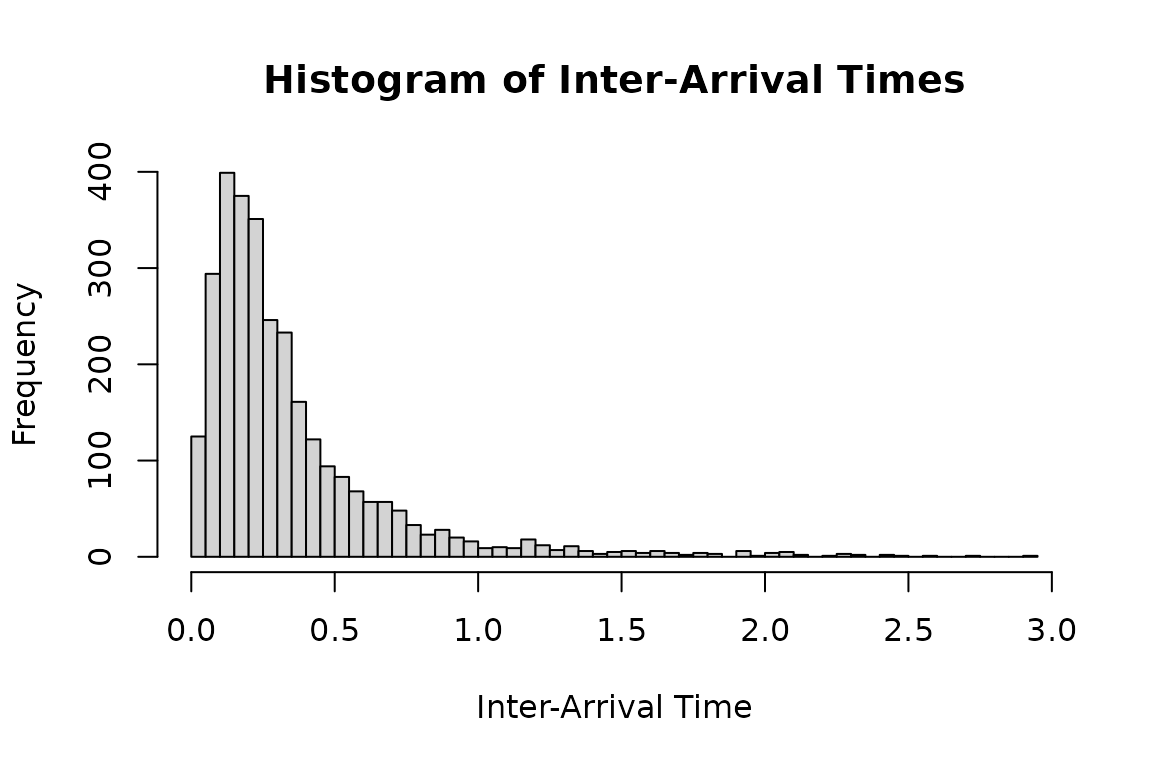
dh1_real <- hsim(hspec1_d, size = 3000)
hist(
  dh1_real$inter_arrival[dh1_real$inter_arrival < 3],
  breaks = 50,
  main = "Histogram of Inter-Arrival Times",
  xlab = "Inter-Arrival Time",
  ylab = "Frequency"
)

This R code snippet demonstrates how to analyze the residual process of a point process model using a flexible distribution. The logLik function is used to compute the log-likelihood of observed inter-arrival times (dh1_real$inter_arrival) based on the distribution specified by hspec1_d. The infer = TRUE parameter allows the function to also infer the residual process, storing the results in infer_res_dh1.

# Infer the residual process using the log-likelihood method
# 'infer_res_dh1' contains the inferred process data based on the inter-arrival times
infer_res_dh1 <- logLik(hspec1_d, inter_arrival = dh1_real$inter_arrival, infer = TRUE)

# Plot a histogram of the inferred residual process
hist(
  infer_res_dh1$res_process1,
  breaks = 100,
  probability = TRUE,
  main = "Histogram of Inferred Residual Process",
  xlab = "Residual Value",
  ylab = "Density"
)

x <- seq(0, 8, 0.1)

lines(
  x,
  dtzexp(x, a = a, ell = ell),
  col = 'red',
  lwd = 2
)

# Add legend for clarity
legend("topright", legend = "Theoretical PDF", col = "red", lwd = 2)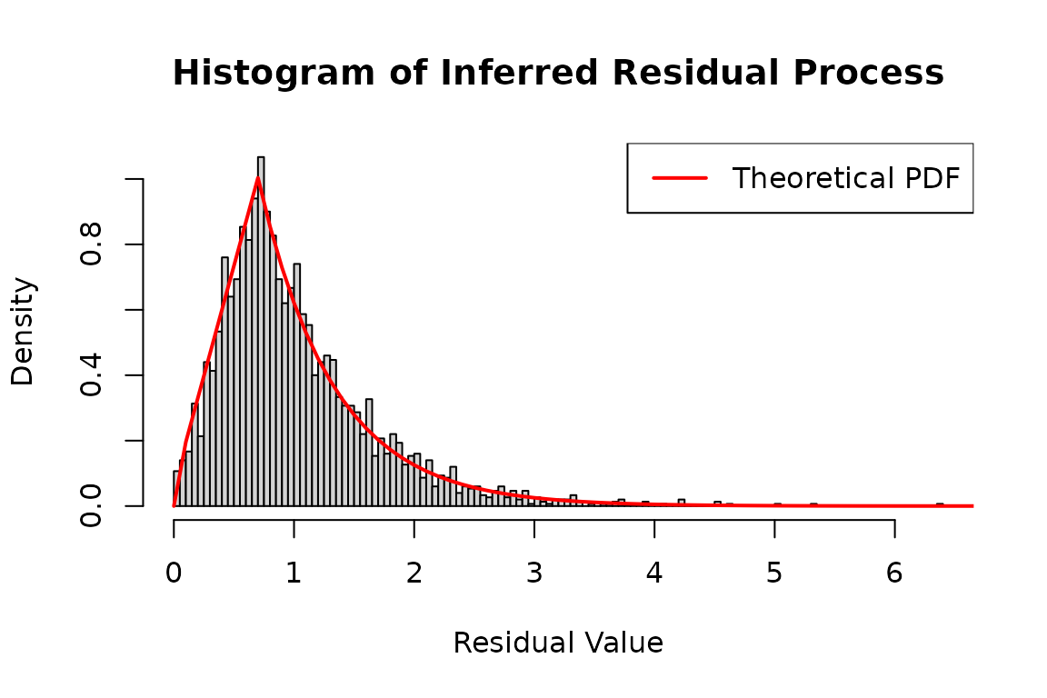

Two-dimenional model

The above method can be extended to multi-dimensions. The basic approach to extension is similar to how multi-dimensional Hawkes models are handled.

mu2_d <- matrix(c(0.3), nrow = 2)
alpha2_d <- matrix(c(0.5, 0.8, 0.8, 0.5), nrow = 2, byrow = TRUE)
beta2_d <- matrix(c(1.5, 1.5, 1.5, 1.5), nrow = 2, byrow = TRUE)
a <- 0.7; ell <- 1.6

hspec2_du <- new("hspec", mu=mu2_d, alpha=alpha2_d, beta=beta2_d,
              rresidual = function(size) rtzexp(n=size, a = a, ell = ell),
              dresidual = function(x, param = c(a = a, ell = ell))
                dtzexp(x, a = param["a"], ell = param["ell"]),
              presidual = function(q, param = c(a = a, ell = ell))
                  ptzexp(q, a = param["a"], ell = param["ell"]),
              qresidual = function(p, param = c(a = a, ell = ell))
                  qtzexp(p, a = param["a"], ell = param["ell"]))
print(hspec2_du)
#> An object of class "hspec" of 2-dimensional Hawkes process
#> 
#> Slot mu: 
#>      [,1]
#> [1,]  0.3
#> [2,]  0.3
#> 
#> Slot alpha: 
#>      [,1] [,2]
#> [1,]  0.5  0.8
#> [2,]  0.8  0.5
#> 
#> Slot beta: 
#>      [,1] [,2]
#> [1,]  1.5  1.5
#> [2,]  1.5  1.5
#> 
#> Slot rresidual: 
#> function (size) 
#> rtzexp(n = size, a = a, ell = ell)
#> 
#> Slot dresidual: 
#> function (x, param = c(a = a, ell = ell)) 
#> dtzexp(x, a = param["a"], ell = param["ell"])
#> 
#> Slot presidual: 
#> function (q, param = c(a = a, ell = ell)) 
#> ptzexp(q, a = param["a"], ell = param["ell"])
#> 
#> Slot qresidual: 
#> function (p, param = c(a = a, ell = ell)) 
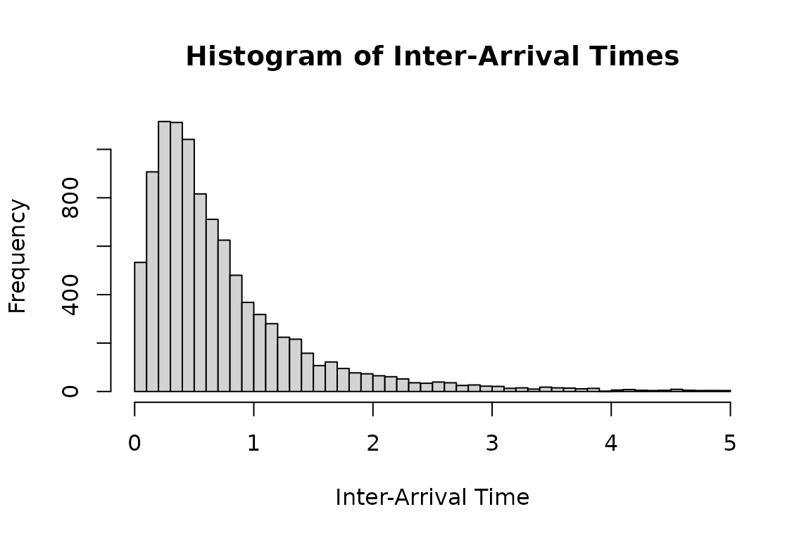
#> qtzexp(p, a = param["a"], ell = param["ell"])

Histogram of inter-arrival times under tzexp distribution.

set.seed(1107)
duh2_real <- hsim(hspec2_du, size = 10000)
# Plot a histogram of the inter-arrival times less than 5
hist(
  duh2_real$inter_arrival[duh2_real$inter_arrival < 5],
  breaks = 50,
  main = "Histogram of Inter-Arrival Times",
  xlab = "Inter-Arrival Time",
  ylab = "Frequency"
)

Inference based on the flexible residual model.

infer_res_dh2 <- logLik(hspec2_du, 
                        inter_arrival = duh2_real$inter_arrival, 
                        type = duh2_real$type, infer = TRUE)

The residual process follows the residual distribution in the model.

# Plot a histogram of the inferred residual process
hist(
  infer_res_dh2$res_process2,
  breaks = 50,
  probability = TRUE,
  main = "Histogram of Inferred Residual Process",
  xlab = "Residual Value",
  ylab = "Density"
)

# Generate a sequence of x values for plotting the theoretical distribution
x <- seq(0, 8, 0.1)

# Add a line to the histogram representing the theoretical density function
lines(
  x,
  dtzexp(x, a = a, ell = ell),
  col = 'red',
  lwd = 2
)

# Add legend for clarity
legend("topright", legend = "Theoretical PDF", col = "red", lwd = 2)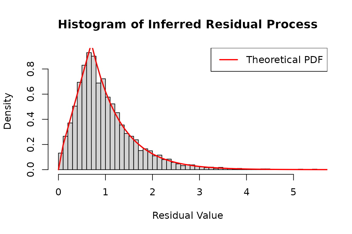

The eres_process follows the exponential distribution.

hist(
  infer_res_dh2$eres_process1,
  breaks = 50,
  probability = TRUE,
  main = "Histogram of Inferred eResidual Process",
  xlab = "Residual Value",
  ylab = "Density"
)

# Generate a sequence of x values for plotting the theoretical distribution
x <- seq(0, 8, 0.1)

# Add a line to the histogram representing the theoretical density function
lines(
  x,
  dexp(x),
  col = 'red',
  lwd = 2
)

# Add legend for clarity
legend("topright", legend = "Theoretical PDF", col = "red", lwd = 2)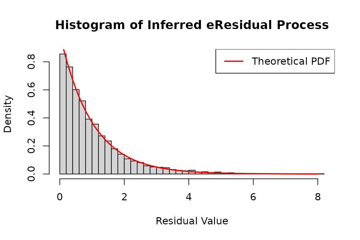

The maximum likelihood estimation.

mle_dh <- hfit(hspec2_du, 
               inter_arrival = duh2_real$inter_arrival, 
               type = duh2_real$type,
               constraint=list(ineqA=rbind(diag(6)), ineqB=matrix(rep(0,6), nrow=6)))
summary(mle_dh)
#> --------------------------------------------
#> Maximum Likelihood estimation
#> BFGS maximization, 68 iterations
#> Return code 0: successful convergence 
#> Log-Likelihood: -12548.98 
#> 6  free parameters
#> Estimates:
#>          Estimate Std. error t value Pr(> t)    
#> mu1      0.289588   0.009073   31.92  <2e-16 ***
#> alpha1.1 0.495306   0.022192   22.32  <2e-16 ***
#> alpha1.2 0.813851   0.024297   33.50  <2e-16 ***
#> beta1.1  1.505598   0.046827   32.15  <2e-16 ***
#> a        0.692895        NaN     NaN     NaN    
#> ell      1.584268        NaN     NaN     NaN    
#> ---
#> Signif. codes:  0 '***' 0.001 '**' 0.01 '*' 0.05 '.' 0.1 ' ' 1
#> 
#> Warning: constrained likelihood estimation. Inference is probably wrong
#> Constrained optimization based on constrOptim 
#> 1  outer iterations, barrier value -0.00051762 
#> --------------------------------------------

Uniform residual distribution example is also provided.

#set.seed(117)
mu2_d <- matrix(c(0.5), nrow = 2)
alpha2_d <- matrix(c(0.3, 0.3, 0.3, 0.3), nrow = 2, byrow = TRUE)
beta2_d <- matrix(c(1.2, 1.2, 1.2, 1.2), nrow = 2, byrow = TRUE)

hspec2_du <- new("hspec", mu=mu2_d, alpha=alpha2_d, beta=beta2_d,
                 rresidual = function(size) runif(n=size, 0, 2),
                 dresidual = function(x, param = c()) dunif(x, 0, 2),
                 presidual = function(q, param = c()) punif(q, 0, 2),
                 qresidual = function(p, param = c()) qunif(p, 0, 2))

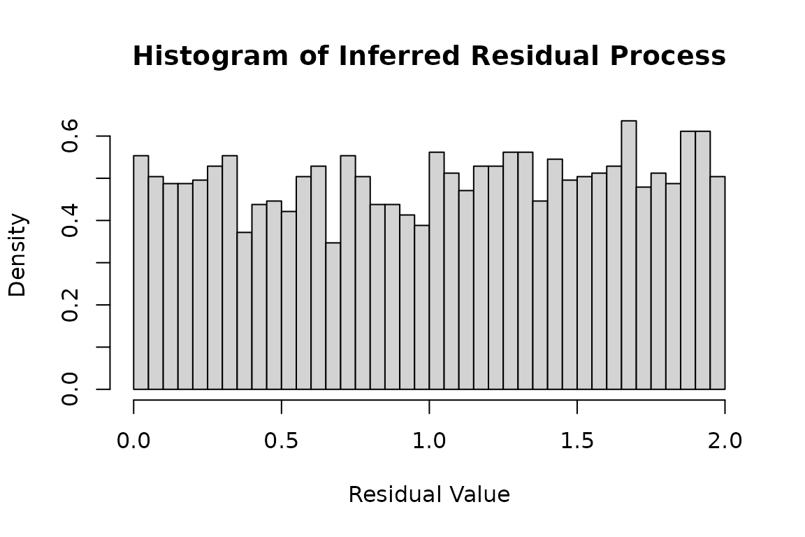
duh2_real <- hsim(hspec2_du, size = 5000)

Histogram of the residual process:

infer_res_duh2 <- logLik(hspec2_du, 
                         inter_arrival = duh2_real$inter_arrival, 
                         type = duh2_real$type, infer = TRUE)

hist(
  infer_res_duh2$res_process1,
  breaks = 50,
  probability = TRUE,
  main = "Histogram of Inferred Residual Process",
  xlab = "Residual Value",
  ylab = "Density"
)